International Journal of Geosciences
Vol.4 No.2(2013), Article ID:28928,7 pages DOI:10.4236/ijg.2013.42028
Impact Estimation and Filtering of Disturbances in FG5 Absolute Gravimeter Observations
Department of Geosciences, School of Natural Sciences and Mathematics, The University of Texas at Dallas, Richardson, USA
Email: *braun@utdallas.edu
Received December 20, 2012; revised January 23, 2013; accepted February 21, 2013
Keywords: FG5 Absolute Gravimetry; Gravity; Disturbance Filtering; Gaussian Bell Summation; Least Squares Adjustment
ABSTRACT
Instrumental and environmental disturbances do affect FG5 absolute gravimeter observations and the estimated gravity values, sometimes to the degree that entire measurement campaigns are discarded. We propose a method which moves towards the re-assessment of previously discarded observations. Once an estimate of the frequency and amplitude of a disturbance in a FG5 data set exists, the proposed method can estimate its impact on the estimated gravity value. This is performed through a Gaussian Bell Summation approach of the functional relationship between disturbance frequency and standard deviation of gravity. The filtering of the identified disturbance is realized through a modification of the functional model of the equation of motion in the least squares adjustment of FG5 observations. The results reveal that the Gaussian Bell Summation approximates the frequency—gravity impact relationship sufficiently well with negligible uncertainties, while the accuracy of the detected disturbance frequency defines a limiting factor for the gravity impact estimation. A realistic disturbance of 15 Hz with an amplitude of 1.5 nm had an impact of ≈48 [μGal] on the gravity estimate. The proposed filter approach reduced the impact to ≈12 [μGal], with the remaining effect being almost entirely associated to the uncertainty in disturbance frequency detection.
1. Introduction
In recent decades, a large amount of FG5 absolute gravimeter data have been accumulated in North America by agencies such as the National Geodetic Survey (USA) and the Geological Survey of Canada. A part of these observations has not been fully exploited yet for different reasons. For example, the FG5 requires an intensive and regular maintenance program and, sometimes, measurements performed at the end of a maintenance cycle are of lower quality. In addition, disturbances (defined as a signal plus noise) during a measurement campaign contaminate absolute gravimeter observations, e.g., signals/ noise caused by construction, microseismicity, or instrumental disturbances. Many studies have addressed individual components of FG5 instrumental or environmental disturbances, cf., [1-4]. Since FG5 observations are very time consuming and costly, the re-assessment of contaminated data through improved de-noising and analysis methods is promising. In addition to the economical aspects, the re-assessment is also beneficial for the gravimetry and geoid communities, which rely on these fundamental observations for calibration or validation of satellite or airborne gravity observations or for the definition of a gravimetric vertical datum. Further, existing time series could be extended and the determination of gravity could be improved [4,5]. It is often the length of the gravity time series which determines its usefulness as temporal changes in gravity are often caused by slow geodynamic processes such as glacial isostatic adjustment [6-8]. The re-assessment of previously discarded FG5 data is the only means to extend a gravity time series back in time. The benefits of being able to filter out detected disturbances are twofold, namely, 1) the determination of gravity is more accurate; and 2) noisy time series of the FG5 observations, which have not been used for analysis due to their high noise level or contamination level could be revitalized.
In this study, we will demonstrate how a detected disturbance in a FG5 time series impacts the estimated gravity value. This approach makes the assumption that a disturbance has been identified in the time series, e.g. using methods such as Lomb-Scargle periodogram analysis or wavelet analysis as demonstrated in [9,10]. A very simple way of filtering out a signal (not considering noise as in a disturbance) from FG5 observations can be achieved by modifying the equation of motion used in the least squares fit, cf., [4,10]. [4,11] proposed a technique which includes a damping factor and a summation over several signals. Herein, no damping factor is included and only one signal is considered at a time. The reason for neglecting a damping factor is because the uncertainty in the required prior frequency detection presents the limiting factor and dominates the damping effects. The analysed time-distance measurements are composed by adding a synthetic signal to a real FG5 data set. This ensures that any real signals originating from the instrument or environment as well as their noise is contained in the data and does not need to be simulated. Only the added signal is perfectly known. This combination allows us to consider the analysed data set as representative for the FG5 measurement process and the following adjustment to estimate gravity.
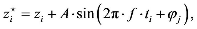
A detected disturbance frequency,  , can be considered by adding a sinusoidal term
to the functional model which modifies to
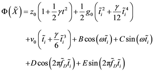 (1)
(1)
Herein,  ,
,  , and
, and  are the unknown initial parameters and
  and
and  are the laser modulation parameters (for details on Equation 1 refer to [10,12,13]). The detected frequency is treated as a ‘true’ parameter (indicated by the tilde), i.e.,
  is not introduced as an unknown parameter which is estimated by the fitting algorithm, cf., the usage of “true” parameter in [14]. However, if Equation (1) is used as a functional model, the following vectors and matrices must be modified within the least squares fit algorithm, cf. [10],
and the design matrix becomes
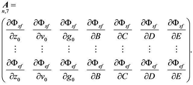
For a signal amplitude of , the approximation values
  and
and  are defined by
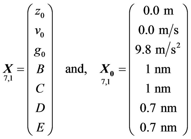
(note that other values could be used, although the results indicate only a small impact of the first guess amplitude). The vector of the estimated unknowns,  , has 7 elements, and it contains
  and
and  from which the amplitude of the signal can be calculated through
and the corresponding phase through .
.
Before starting a time consuming reprocessing with a modified observation equation for large amounts of data, it is beneficial to investigate what level of improvement can be achieved. In other words, if a signal in a data set was detected, e.g., by spectral analysis tools such as Lomb-Scargle or wavelets [10], an estimation of its impact on the derived gravity value would enable the quantification of potential improvements through filtering, an initial step in the process of re-assessment. In this study, we present a numerical tool for the estimation of the disturbance signal impact on gravity. There are multiple ways of filtering a detected disturbance in order to decrease its impact on gravity estimates. Herein, only one filtering approach is presented, as the focus of this study lies on the impact assessment. This includes the important consideration that the FG5 observations at hand first go through the transfer function of the FG5 measurement process, then through an adjustment process, before estimating a gravity value. In order to keep most of these processes in the impact assessment, we used real observations together with known synthetic disturbances in this study.
The FG5 data used herein were provided by Natural Resources Canada. The measurements used in the text were collected July 8, 2008 at the Pacific Geoscience Centre in Sidney, British Columbia, Canada. A data subset of 100 drops was used for most computations (FG5#236: file 2008a0708 ({*}.raw, {*}.project), Sets 37-40, 25 Drops/Set, total 100 Drops).
2. Signal Impact Analysis
For the following synthetic analysis a real FG5 data set of 100 drops with all time-distance measurements,  and
and![]() , was used. The 100 drops were analyzed before by Lomb-Scargle Periodogram analysis to be sure that no significant disturbance exists in the data set [9]. A sinusoidal signal was added to the distance measurement
, was used. The 100 drops were analyzed before by Lomb-Scargle Periodogram analysis to be sure that no significant disturbance exists in the data set [9]. A sinusoidal signal was added to the distance measurement
 (2)
(2)
where  is the amplitude in
  and
and  the signal frequency in
 . Further, in Equation (2) the index
  denotes the used fringes,
 . Furthermore, from drop to drop the phase was chanced to cover the range of
  within the 100 drops. Hence, the phase is defined by
with . A full parameter space study of how sensitive the FG5 measurement and adjustment process is for varying disturbance frequency, amplitude and phase was performed in [9]. We used the results of that study for defining relevant frequencies, amplitudes and phase. A least squares fit was performed for the 100 drops with both types of distances (without an added signal
  and with an added signal
 ). This can be expressed by

![]()
The differences between each pair of affected and unaffected gravity estimates were computed for each drop, i.e.,

and the standard deviation of the set of differences
was calculated. This analysis was performed for the set of frequencies  given in
 . Figure 1 shows the results of a frequency analysis up to 100 [Hz] with three different amplitudes. It also validates the results of [15] and provides an analysis tool similar to the results of [16], who have conducted a similar impact analysis for geodetic velocity estimation. The most important conclusions from analyzing Figure 1 are: 1) the lower signal frequencies have the largest impact on gravity; and 2) small changes in frequency can have significantly different impacts on gravity. These facts are caused intrinsically by the way the FG5 transfers a disturbance to time-distance measurements and finally to the gravity estimate. It is worth to note that changing the number of selected fringes will lead to a different drop frequency, cf equation in next page, which in turn will change the impact on gravity. Hence, the curves in Figure 1 must be re-evaluated every time, the fundamental parameters drop frequency, number of drops, selected start and end fringes, amplitude and phase change.
3. Estimation of Signal Impact on Gravity
In order to perform the task of data re-assessment in an effective manner, a tool for the estimation of the signal impact on gravity is very useful. Figure 1 shows the frequency sensitivity of the FG5 and its impact on gravity. Since the standard deviation is based on a set of gravity
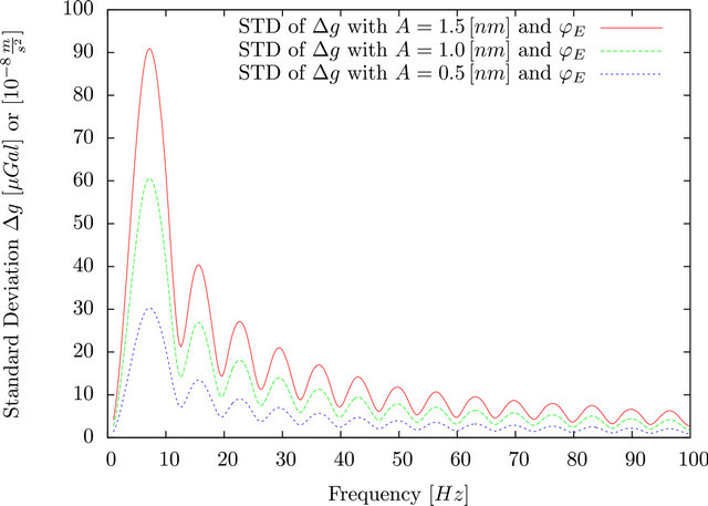
Figure 1. Impact of signal frequency on gravity estimation in the FG5 observation process. Data used: FG5#236, file 2008a0708, sets 37-40, (25 drops/set, total 100 drops).
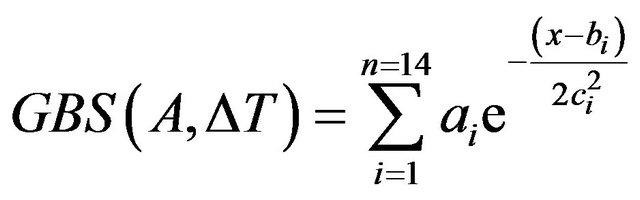
differences, not on absolute values, the plot is of a general character. Figure 1 can be used to estimate the impact on gravity for a detected frequency,  , and for a certain amplitude, which has to be estimated. Since the curves in Figure 1 have a distinct shape and are continuously differentiable, it should be possible to find an appropriate approximation using analytical functions. It is obvious that this desired function depends on the disturbance amplitude and drop period/frequency. Furthermore, it seems possible that the curves shown in Figure 1 can be approximated by a summation of several Gaussian bells. In general, the Gaussian bell summation
  is given by
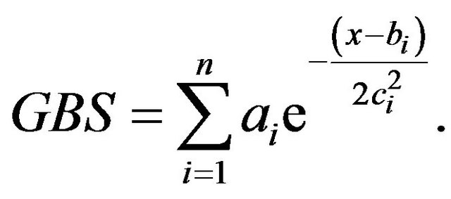 (3)
(3)
In order to determine a relationship between the Gaussian parameters  and the amplitude of the disturbance
  (in [nm]) and the drop period
(the subscripts  and
and  refer to the start fringe and end fringe), several curves as in Figure 1 with different amplitudes and drop periods were analyzed. A parameter space of
  in
in ,
,
 in
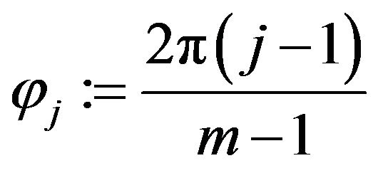
in  was used. For each constellation of amplitude and frequency the phase was evenly spread between, i.e.,
where  is the drop index and
 ![]() the number of used drops. With this parameter space, the curves were generated and a least squares fit for each curve was performed to obtain the three parameters for each Gaussian bell. The results for each parameter were analyzed. The heuristically identified relationship between
the number of used drops. With this parameter space, the curves were generated and a least squares fit for each curve was performed to obtain the three parameters for each Gaussian bell. The results for each parameter were analyzed. The heuristically identified relationship between
is described by
 (4)
(4)
with
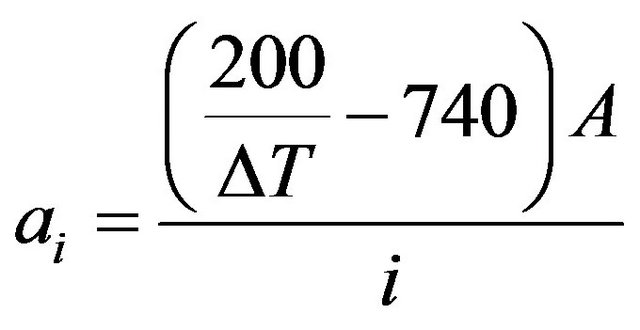
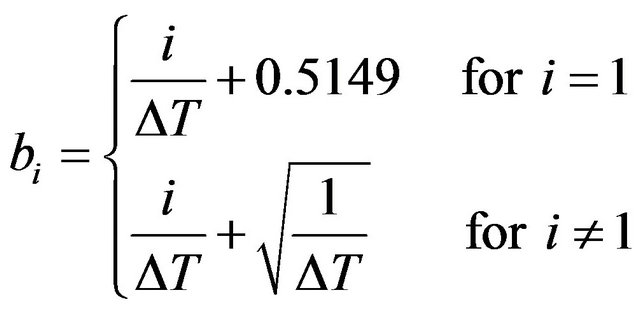
and is valid for frequencies up to , which corresponds to a summation of
  Gaussian bells. Parameter
  corresponds to the amplitude of the
  -th Gaussian bell, and is controlled by the amplitude of the synthetic signal and the drop period used. Parameter,
 ![]() , describes the position of the center of each Gaussian bell. A closer look reveals that the first peak is not exactly at the drop frequency
, describes the position of the center of each Gaussian bell. A closer look reveals that the first peak is not exactly at the drop frequency
 but has a shift of
  on average. It is very likely that this is caused by the intrinsic data window of the FG5 observations. A periodic behavior of this shift was detected between
 , and it depends on the drop period used. The differences over the fringe space of
are shown in Figure 2. For the sake of convenience, the average of  was taken to keep Equation (4) simple. Parameter
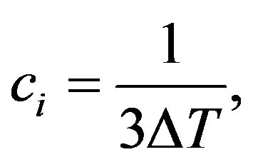
 ![]() controls the width of each Gaussian bell. Since local maxima are around the multiples of
controls the width of each Gaussian bell. Since local maxima are around the multiples of , the space between two local maxima can be well approximated by
 and hence
  of this length is taken to define each bell width. In Figure 3, the
  approximations are shown for two different amplitudes and for two different
 . In general, the approximation at the beginning is worse than at the end; this can be observed in the second maximum in each subplot. However, this discrepancy is acceptable, since the goal is to estimate the impact on gravity, and also the disturbance amplitude. Pseudo-Voigt functions representing sums of Gaussian and Lorentzian functions [17,18] were tested instead of Gaussian bells, which provided a better approximation. However, this introduced more parameters, which made it much more difficult to find a relationship between the parameters,
  and the signal amplitude.
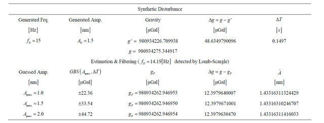
In Table 1, a numerical example for a single drop is given. The generated synthetic signal of  with an amplitude of
  has an impact on gravity value of
 . With Lomb-Scargle and filtering via Equation (1) the impact can be reduced considerably to
 . The remaining difference is caused by the fact that Lomb-Scargle is not able to detect the exact frequency of
 , cf. [9]. The results of the esti-
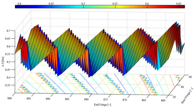
Figure 2.  is the difference of frequency at the first peak (in the plot of standard deviation analysis of
 , cf., max peak in Figure 1) and
  depending on the start and end fringes used. Data used: FG5#236, file 2008a0708, sets 37-40, (25 drops/set, total 100 drops).
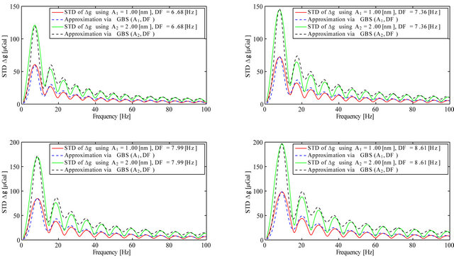
Figure 3. The four panels show the standard deviation of  and its approximation for two different
  (
( and
and ) and two different amplitudes (
 and
and ). Data used: FG5#236, file 2008a0708, Sets 37-40, (25 drops/set, total 100 drops).
Table 1. Numerical example of impact estimation and filtering. The upper table contains information about generated signal, the lower table presents the numerical results of estimation and filtering. The not affected gravity value is indicated by , the affected by
 . Both are calculated through a least-squares adjustment. Lomb-Scargle analysis was used to estimate
  for the drop residuals; Equation (1) was used to filter out
 . The obtained estimated gravity is
 , and the estimated amplitude is
  Further, the number of digits are extended to point out the small differences in the results. Data used: FG5#236, file 2008a0708, set 37, drop 1.
mation via the  Equation (4) are acceptable and the misfit described in Figure 3 has a negligible impact on gravity compared to the limitations in frequency detection using Lomb-Scargle. Because of the strong slope of the
  function at this point, a difference of 0.5 [Hz] at around 15 [Hz] causes a change in gravity of 11.8[μGal]. This value is very close to the remaining difference after filtering of
 , with
 .
.
The numerical example in Table 1 demonstrates that the filtering efficiency depends mostly on the detection accuracy. The guessed amplitude has a minor impact on  and can be considered as very robust.
4. Conclusion
A Gaussian Bell Summation  was developed to approximate the frequency dependent impact of disturbances on gravity estimates (Figure 1 and 3). The approximation requires only two parameters, the drop period
 , and a rough estimate of the disturbance amplitude,
 . In addition to the analytical term, a numerical comparison of
  estimation and filtering is made for a single drop to demonstrate the
  performance. The filter is realized by a modification of the FG5 least-squares observation equation and uses the detected frequency as a “true observation” in the adjustment algorithm. The modified least-squares fit algorithm estimates the unknown amplitude of the signal quite well and does not depend on the guessed initial amplitude value. The developed
  can be used to obtain estimates of the impact of known or detected disturbances on gravity. It is a useful tool for the re-assessment of previously discarded FG5 observations. It can be used to improve the estimated gravity values markedly. The limiting factor of this approach is the uncertainty in disturbance frequency detection, e.g. by using Lomb-Scargle periodogram analysis, which prevends the proposed filter to remove all of the disturbance impact. Initial tests using a disturbance frequency detection algorithm based on wavelets [10] shows improved accuracy and would further reduce the gravity impact of detectable disturbances.
5. Acknowledgements
The authors are grateful for input and discussions with Joseph Henton and Nicholas Courtier (Pacific Geoscience Centre, Geological Survey of Canada, Sidney, British Columbia, Canada). FG5 data used herein were kindly provided by Natural Resources Canada.
REFERENCES
- H. Hanada, T. Tsubokawa and S. Tsuruta. “Possible Large Systematic Error Source in Absolute Gravimetry,” Metrologia, Vol. 33, No. 2, 1996, pp. 155-160. doi:10.1088/0026-1394/33/2/4
- G. Durando and G. Mana, “Propagation of Error Analysis in a Total Least-Squares Estimator in Absolute Gravimetry,” Measurment Science & Technology, Vol. 13, No. 10, 2002, pp. 1505-1511. doi:10.1088/0957-0233/13/10/301
- C. Rothleitner and O. Francis, “On the Influence of the Rotation of a Corner Cube Reflector in Absolute Gravimetry,” Metrologia, Vol. 47, No. 5, 2010, pp. 567-574. doi:10.1088/0026-1394/47/5/007
- F. J. Klopping, G. Peter, D. S. Robertson, K. A. Berstis, R. E. Moose and W. E. Carter, “Improvements in Absolute Gravity Oberservations,” Journal of Geophysical Research, Vol. 96, No. B5, 1991, pp. 8295-8303. doi:10.1029/91JB00249
- M. van Camp, S. D. P. Williams and O. Francis, “Uncertainty of Absolute Gravity Measurements,” Journal of Geophysical Research, Vol. 110, No. B5, 2005.
- A. Lambert, N. Courtier and T. S. James, “Long-Term Monitoring by Absolute Gravimetry: Tides to Postglacial Rebound,” Journal of Geodynamics, Vol. 41, No. 1-3, 2006, pp. 307-317. doi:10.1016/j.jog.2005.08.032
- S. Mazzotti, A. Lambert, N. Courtier, L. Nykolaishen and H. Dragert, “Crustal Uplift and Sea Level Rise in Northern Cascadia from GPS, Absolute Gravity, and Tide Gauge Data,” Geophysical Research Letters, Vol. 34, No. 15, 2007, 5 p.
- S. D. P. Williams, T. F. Baker and G. Jeffries, “Absolute Gravity Measurements at UK Tide Gauges,” Geophysical Research Letters, Vol. 28, No. 12, 2001, pp. 2317-2320. doi:10.1029/2000GL012438
- M. Orlob and A. Braun, “On the Detectability of Synthetic Disturbances in FG5 Absolute Gravimetry Data Using Lomb-Scargle Analysis,” Geomatica, Vol. 66, No. 2, 2012, pp. 113-124. doi:10.5623/cig2012-024
- M. Orlob, “Spectral Analysis of Synthetically Affected FG5 Absolute Gravimeter Residuals,” Ph.D. Thesis, Department of Geosciences, The Univsersity of Texas, Dallas, 2011.
- K. Charles and R. Hipkin, “Vertical Gradient and Datum Height Corrections to Absolute Gravimeter Data and the Effect of Structured Fringe Residuals,” Metrologia, Vol. 32, No. 3, 1995, p. 193. doi:10.1088/0026-1394/32/3/007
- MicroG-Lacoste, “FG5 g8 User’s Manual/Software,” MicroG-Lacoste, Erie, 2008.
- T. M. Niebauer, G. S. Sasagawa, J. E. Faller, R. Hilt and F. Klopping, “A New Generation of Absolute Gravimeters,” Metrologia, Vol. 32, No. 3, 1995, pp. 159-180. doi:10.1088/0026-1394/32/3/004
- W. Niemeier, “Ausgleichsrechnung,” 1 Edition, Walter de Gruyter, Berlin, 2002.
- L. Timmen, R. Röder and M. Schnüll, “Absolute Gravity Determinations with JILAG-3—Improved Data Evaluation and Instrumental Technics,” Bulletin Géodésique, Vol. 67, No. 2, 1993, pp. 71-81. doi:10.1007/BF01371370
- G. Blewitt and D. Lavallee, “Effect of Annual Signals on Geodetic Velocity,” Journal of Geophysical Research, Vol. 107, No. B7, 2002, pp. ETG 9-1-ETG 9-11. doi:10.1029/2001JB000570
- J. J. Olivero and R. L. Longbothum, “Empirical Fits to the Voigt Line Width: A Brief Review,” Journal of Quantitative Spectroscopy and Radiative Transfer, Vol. 17, No. 2, 1977, pp. 233-236. doi:10.1016/0022-4073(77)90161-3
- “NIST Handbook of Mathematical Functions,” Cambridge University Press, Cambridge, 2010.
NOTES
*Corresponding author.