Journal of Flow Control, Measurement & Visualization
Vol.2 No.2(2014), Article ID:44768,13 pages DOI:10.4236/jfcmv.2014.22007
Investigation of Unsteady Flow Fields for Flow Control Research by Means of Particle Image Velocimetry
Reinhard Geisler, Andreas Schröder, Jürgen Kompenhans
Department of Experimental Methods, Institute of Aerodynamics and Flow Technology, German Aerospace Center (DLR), Göttingen, Germany
Email: reinhard.geisler@dlr.de
Copyright © 2014 by authors and Scientific Research Publishing Inc.
This work is licensed under the Creative Commons Attribution International License (CC BY).
http://creativecommons.org/licenses/by/4.0/


Received 14 January 2014; revised 4 March 2014; accepted 12 March 2014
ABSTRACT
Unsteady three-dimensional flow phenomena must be investigated and well understood to be able to design devices to control such complex flow phenomena in order to achieve the desired behavior of the flow and to assess their performance, even in harsh industrial environments. Experimental investigations for flow control research require measurement techniques capable to resolve the flow field with high spatial and temporal resolution to be able to perceive the relevant phenomena. Particle Image Velocimetry (PIV), providing access to the unsteady flow velocity field, is a measurement technique which is readily available commercially today. This explains why PIV is widely used for flow control research. A number of standard configurations exist, which, with increasing complexity, allow capturing flow velocity data instantaneously in geometrical arrangements extending from planes to volumes and in temporal arrangements extending from snapshots to temporarily well resolved data. With increasing complexity these PIV systems require advancing expertise of the user and growing investment costs. Using typical problems of flow control research, three different standard PIV systems will be characterized briefly. It is possible to upgrade a PIV system from a simple planar to a “high end” tomographic PIV system over a period of time, if sufficient PIV expertise can be built up and budget for additional investments becomes available.
Keywords:Flow Control, Flow Velocity, Particle Image Velocimetry, Stereo PIV, Tomographic PIV

1. Introduction
Flow control involves passive or active devices to affect a beneficial change in wall-bounded or free shear flows [1] . Active control (see [2] and [3] for example), where the actuator is located in a region sensitive to the phenomenon to be controlled, is of increasing interest. Research and development activities requiring flow control technology employ theoretical, experimental and numerical methods. As far as experimental methods are concerned, there is the need to be able to capture the structures of the flow field instantaneously to understand and assess flow control phenomena.
Since two decades technological progress at lasers, video techniques, optoelectronics, computers and evaluation algorithms allows to extract quantitative information from images of flows. Continuous improvement of such image based measurement techniques and decreasing costs of equipment enabled many research groups to exploit these techniques for obtaining 2-dimensional or even 3-dimensional data mainly for fundamental research. Since a decade ago many image based measurement techniques have found interest in industrial applications and are even used as a matter of routine when trying to improve the understanding of complex flow phenomena. In particular, Particle Image Velocimetry (PIV), which allows determining the velocity information at many locations within an unsteady flow field simultaneously by two times illuminating small tracer particles in the flow within a few microseconds, has found widespread use by researchers at universities and in industry. The fundamental principles of the PIV technique are explained in textbooks [4] [5] in detail, the present state-ofthe-art can be found in journals or conference proceedings.
Scientists investigating flow control phenomena are primarily interested in understanding and assessment of devices and methodologies to control the behavior of unsteady, three-dimensional flows, being wall-bounded or free shear flows, which requires temporally and spatially well resolved qualitative and quantitative information of the flow volume under consideration. In case of flow control involving flexible or moving walls the knowledge of the shape and deformation of the walls is needed in addition. All data must be acquired non-intrusively so that no interference of the flow field by the measurement is to occur. The availability of such high quality experimental data does not only provide insight into the fluid mechanical phenomena involved in controlling the flow but also supports the validation of the results of numerical calculations.
In summary, the most important features of an appropriate measurement technique to study flow control phenomena in fluid mechanics or aerodynamics can be described as follows:
1) Application in air and water flows with periodic, repetitive or chaotic behavior.
2) Application in boundary layer flows, shear flows, wakes, vortical flows, channel/pipe flows, cylinders, jets, ribs to enhance mixing, etc.
3) Non-intrusive methods, no interference of measurement with flow control phenomena to occur.
4) Instantaneous velocity data, captured simultaneously everywhere in the observation field.
5) Resolution of small as well as of large scale structures depending on phenomenon of interest.
6) Stimulation of the flow field on extremely short length and time scales (e.g. by MEMS) near the critical flow regimes, where flow instabilities magnify quickly, requires high spatial and temporal resolution of velocity data to be able to study the development of the essential structures within the flow field (delaying/advancing of transition, suppressing/enhancing turbulence, preventing/ provoking separation [1] ).
7) Triggering of velocity measurement relative to the operation cycle of the actuators for active flow control.
PIV having become a mature technique, scientists interested in flow control problems are rather end users than developers of the PIV technique. As such, when designing a flow control experiment and selecting a PIV system, very often they may not be aware of all implications provided by the selected equipment on the data which can be measured.
The main features of the PIV technique to be observed when dealing with flow control are:
1) Instantaneous measurement: a large flow field can be captured simultaneously within a few microseconds.
2) Imaging systems with different magnification allow observing small as well as large scale structures.
3) In principle the velocity field is captured within a (laser) plane (2D). Nowadays, also 3D (tomographic) techniques are available, which, however, require higher experimental effort.
4) The performance of the PIV system is determined by the selection of the kind of illumination system (cw lasers, pulse lasers, flash lamps, LED illuminators), cameras (temporal and spatial resolution) and the number of illumination and camera systems available.
5) Depending on the PIV set-up, two (2C) or three (3C, stereo configuration) components of the velocity vector can be measured.
6) PIV works non-intrusively, but requires tracer particles to determine the flow velocity. These tracer particles must follow the flow faithfully. Thus, in water flows, bigger particles can be utilized, which scatter more light than the particles of a diameter of 1 μm, which are usually used in air flows. This means that experimental requirements (and costs) are more relaxed for PIV applications in water than in air.
7) Depending on the light source utilized some minimum time delay is required between two successive PIV measurements (recording frequency of standard Nd:YAG laser based PIV systems: 10 - 20 Hz (~snapshots); recording frequency of high-speed PIV systems: 1 - 5 kHz, which may allow a temporally resolved measurement, depending on flow phenomena). It must be pointed out that standard PIV systems are more powerful and allow to illuminate a larger observation field.
8) Employing appropriate hardand software [6] the triggering of a PIV recording relative to an external event is possible.
The explanations given above make clear that there does not exist a “one fits to all” PIV system. Figure 1 (see [4] for further explanations) summarizes the most essential features of PIV systems with respect to their spatial and temporal resolution. Today’s CCD cameras offer a somewhat higher number of pixels and repetition rate; however the basic relations explained in Figure 1 are still valid. Recently, some special devices and arrangements, based on profound knowledge of optics, allow experienced users to extend the size of the observation area above those figures as given in Figure 1.
Based on the considerations made above and as example for the potential of image based measurement techniques applied to flow control, an overview of the measurement of flow velocities employing different configurations of PIV systems will be given next. The performance of PIV systems such as planar PIV, stereoscopic PIV, tomographic PIV and corresponding modifications utilizing high-speed cameras for recording to achieve the required temporal resolution will be presented and their application to flow control research will be described briefly. For each configuration topics such as required equipment, complexity of operation, information to be gained, operational problems etc. will be discussed based on the experiences made at such applications for fundamental research or within industrial projects by the Department of Experimental Methods of the Institute of Aerodynamics and Flow Technology of the German Aerospace Center [7] or together with partners, respectively.
2. PIV Systems
2.1. Two Component-Two Dimensional PIV System (2C-2D PIV)
The development of PIV started in the 1980s with 2C-2D PIV systems, i.e. one camera, one illumination source, and a planar illumination (light-sheet). The focus of the scientific work concentrated on seeding problems, particle scattering, following behavior of tracer particles, development of evaluation algorithms, accuracy etc. The PIV plane was arranged in direction of the main flow, in order that the tracer particles do not leave the light-
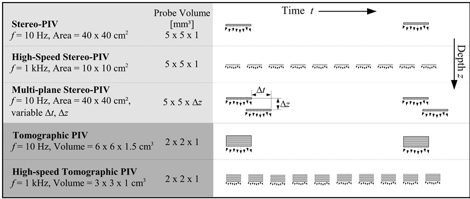
Figure 1. Schematic overview over present variants of the PIV method with their typical spatial and temporal resolution. The symbols present the measurable three-component velocity vectors for each method in their spatial and temporal arrangement [4] .
sheet in between the two illuminations, which would not allow obtaining PIV data. A small misalignment of the light-sheet plane and the main flow direction would lead to measurement errors. Also it was recognized that under certain imaging conditions so-called perspective errors will occur. With the development of robust stereo PIV systems, i.e. two cameras and a planar illumination (see Chapter 2.2) such problems could be avoided and stereo PIV became the standard PIV configuration for the investigation of complex flow phenomena.
Today the use of 2C-2D PIV systems, which are the simplest, easy to use and cheapest ones, is only recommended if:
1) The flow field is nearly two-dimensional.
2) The object to be investigated allows only one viewing direction (e.g. due to restrictions by walls).
3) The PIV measurement shall serve to obtain an overview of an unknown flow field (location and size of structures, range of spatial and temporal scales etc.) before a more complex and costly investigation will start.
4) The PIV measurement shall check the seeding quality, tracer behavior, functionality of PIV system, e.g. with respect to triggering to an external event, functionality of external devices (structural performance of PIV set-up (due to vibration, noise), model vibrations, operated model movements, actuators etc.).
If due to lack of equipment a 2C-2D PIV system must be used for research the above mentioned problems involved in the use of such an arrangement should be minimized for the experiment and their remaining implications on the results must be discussed in the publication.
The required knowledge of optics, lasers, image processing, video technique etc. as well as the complexity of the hardand software of PIV systems increase from 2C-2D systems to stereo and tomographic systems, requiring advancing expertise and growing investment. Thus, for persons starting to use the PIV technique it is recommended to begin with a 2C-2D PIV system in order to familiarize themselves with the technique and to understand its fundamental principles, to characterize and optimize the flow facility and the seeding with tracer particles, the light-sheet optics and the imaging system, to avoid background light or light scattering from surfaces, to learn the laser safety procedures, to develop a reliable calibration procedure for the whole system, to check and optimize the internal triggering of the PIV system and its connection to external events, to get familiar with the evaluation software and the post processing of the data and to check the accuracy of the obtained data and to validate them.
The use of a 2C-2D PIV system will be described next taking a generic aeroelastic experiment [8] to explore the flutter of a thin plate under unsteady aeroelastic forces as an example. In a later stage the control of flutter may also be a topic of research activities. The present objectives were to set-up an experimental system to measure the velocity of the flow field and the deformation (location and acceleration) of the thin plate simultaneously and time resolved to study the interactions among inertial, elastic and aerodynamic forces acting on the structure. For measurement of the deformation of the thin plate the Image Pattern Correlation Technique IPCT [9] was utilized. IPCT observes the movements of a random dot pattern imprinted on the surface of the thin plate to determine the deformation of the plate. In order to assess the performance of the combined PIV and IPCT high-speed measurements it was considered to be sufficient to use a 2C-2D-T PIV system to reduce the complexity of the set-up. This is justified by the fact, that the flow is nearly two-dimensional. The PIV system consisted of a diode-pumped Nd:YAG laser (20 mJ per pulse at 5 kHz) and a 4 megapixel high-speed CMOS camera with 5 kHz framing rate at reduced resolution (1344 × 688 pix). The observation area was 66 × 130 cm2, the spatial resolution 0.6 × 0.6 mm2. DEHS tracer particles of 1 μm diameter were used for seeding the flow. The IPCT system consisted of two CMOS cameras in Scheimpflug mounts and two LED illuminators developed at DLR [10] . Figure 2 shows a sketch of the experimental set-up with two high-speed cameras to determine the deformation of the fluttering plate and a third high-speed camera (not depicted here) to observe the flow field to determine the velocity within the marked rectangular field of view. The measurement plane is illuminated from two directions using overlapping light sheets to prevent shadowing effects by the plate. For further technical details, such as illumination optics and triggering see [8] . As examples of the quality of results, which can be obtained, one instantaneous velocity vector field (Figure 3) and one instantaneous surface of the fluttering plate (Figure 4) are presented. Now, the data obtained with this experimental set-up of limited complexity allow to calculate local and integral elastic forces from position measurements derived from single-shot IPCT data, to calculate local and integral inertia forces from the time derivative of the surface velocity and respective mass distribution, to calculate the aerodynamic forces by integration of the pressure term in the Navier-Stokes-Equation by assuming 2D-flow, and, finally, to compare the calculated forces with respect to the 2D-flow assumption,
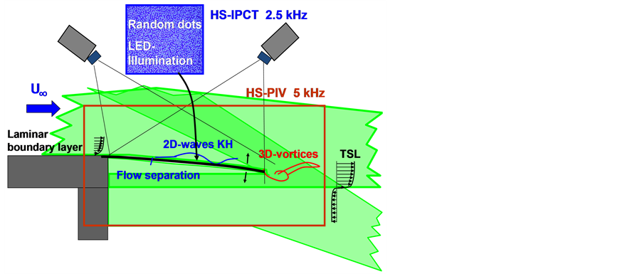
Figure 2. Experimental set-up: High-speed PIV system and high-speed IPCT system with thin plate.
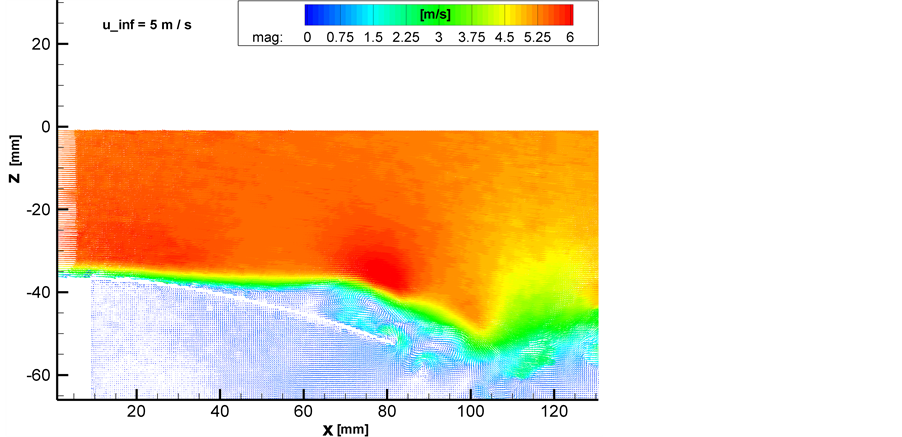
Figure 3. Instantaneous velocity field for one flutter case.
noise sources etc. Once this approach has proven to be successful, more complex experimental set-ups may be used (tomographic PIV).
Finally, some information shall be provided on the resources needed to perform such an experiment. The cost of this PIV related equipment (high-speed PIV system requiring high-speed lasers and high-speed cameras) is about 160% of that of a standard (snapshot) 2C-2D PIV system. In order to perform the experiment a man power of about 12 person months was required. The researcher responsible for the PIV experiment should have already carried out several complex PIV measurements, which will require an experience of about 24 person months.
2.2. Three Component-Two Dimensional (Stereo) PIV System with Temporal Resolution (3C-2D-T PIV)
To upgrade a PIV system from a 2C to a 3C system, in addition, a second camera is needed, two Scheimpflug mounts to keep the images of the tracer particles in focus for an oblique arrangement of the cameras and 3C PIV evaluation software. If the 2C-2D PIV system has been optimized as described in chapter 2.1 and can be operated routinely, then—in particular—the following topics need to be addressed for operation of a 3C-2D PIV system:
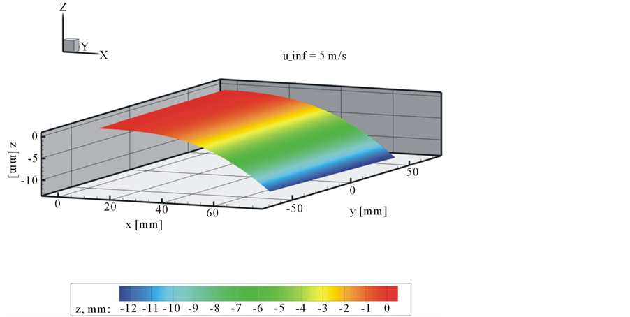
Figure 4. Instantaneous surface of thin plate for one flutter case.
1) Operation of Scheimpflug mounts (one or more axes)
2) More complex calibration of the arrangement of measurement plane, light-sheet plane, Scheimpflug mounts, and cameras. As data obtained by two cameras need to be combined to calculate the third velocity component, misalignments will lead to artifacts (e.g. distortion of the shape of vortices). Thus, such calibration algorithms need to be well understood and calibration procedures need to be well trained as any mistake during calibration cannot be recovered later.
3) Understanding of scattering behavior of the tracer particles. With two cameras the first one is located in forward and the second one in backward scattering direction in most cases, which leads to different level of intensity of the scattered light.
4) Robust construction of recording set-up, to minimize effects of vibrations such as defocusing or individual movement of each of the two cameras, which would deteriorate the 3C results. Today to some limit the re-arrangement of PIV recordings captured by vibrating cameras can be done by software after the measurement.
5) Measurements in planes perpendicular to the main flow direction require the possibility to modify the light-sheet optics in order that the plane of the first and the second illumination can be displaced.
If these problems have been solved the 3C-2D PIV system can be routinely used for fundamental research and industrial development. The huge number of data possible to capture with such a system will require fast evaluation algorithms, fast computers and big data storage.
One possible upgrade of a single 3C-2D PIV system would be to operate two 3C-2D PIV systems simultaneously, to 1) Extend the observation areas (placing the systems side by side)
2) Image with different magnification for each of the systems to be able to resolve large and small scale spatial structures simultaneously 3) Place the two systems in the same or in a slightly displaced plane to follow the spatial and temporal evolution of structures (for application in air, this usually requires to make use of differently polarized light for illumination to be able to separate the light scattered by the tracer particles for each illumination)
The upgrade for two 3C-2D PIV systems would require a doubling of the components (laser, cameras, Scheimpflug mounts) and more or less a doubling of cost.
Standard 3C-2D PIV systems for air flows use Nd:YAG lasers for illumination (pulses of 200 mJ to 400 mJ at 10 ns pulse width and λ = 532 nm). These lasers allow illuminating quite a large area of the flow but do not allow taking recordings with a frequency of more than 10 or 15 Hz (“snapshots”, see Figure 1). Velocity vector maps taken with such a temporal resolution can either be analyzed statistically or—in case of repetitive or periodic events—the method of conditional sampling can be applied.
However, for many fluid mechanical problems including flow control research a higher temporal resolution is desired to be able to follow the temporal behavior of individual structures. This can be done with some limitations by upgrading to a 3C-2D-T PIV system. Such a system requires the purchase of a special laser and special cameras with higher repetition rate (up to a few kHz). The disadvantage of such a 3C-2D-T PIV system is that the laser power is less and, thus, only a much smaller observation area can be covered than with a standard 3C-2D PIV system (compare Figure 1). This means, for general demands, both, a 3C-2D standard PIV system and a 3C-2D-T PIV system should be available for a research group investigating flow control problems.
To illustrate the potential of PIV for flow control research an application with two 3C-2D-T PIV systems has been selected. The scientific problem to be investigated was to characterize pulsed and continuous jet actuators in a turbulent boundary layer [11] [12] . The test aimed at generating an aerodynamic data base useful for the characterization of (unsteady) vortical structures in the wake of a jet actuator row and at comparing the efficiency of continuous and pulsed jet vortex generators. The objective was to study the flow field behind the actuators and further downstream where the effect of the actuators could be identified and assessed. The data set should also be used for the validation of CFD tools or simplified models for jet vortex generators. In a joint measurement campaign of the French and German research organizations for aerodynamics and aeronautics, ONERA and DLR, each having available a high-speed PIV system, it was possible to combine both systems to capture the velocity data in both areas of interest simultaneously (see Figure 5 and Figure 6), which would not have been possible with a single system.
The observation area having a size of 78 mm × 40 mm, the flow velocity being in the range of 15 m/s to 30 m/s, the pulse frequencies of the jets being 50 Hz and 100 Hz, and olive oil droplets of a diameter of 1 μm as tracer particles, two high-speed PIV systems with two oscillators each supplying two consecutive pulses at 1 kHz with about 20 mJ per pulse were used. Combination of a frequency-doubled Nd:YLF laser (at λ = 527 nm) and a Nd:YAG laser (at λ = 532 nm) did not provide problems. The layout of the trigger electronics and the timing diagram are presented in Figure 7 and Figure 8.
The time interval between each of the two light pulses has been adjusted in the frame straddling mode according to the measured flow dynamics between τ = 30 µs and 80 µs. For the recording of PIV images, highspeed CMOS cameras (1024 × 1024 pix @ 3 kHz with 10 bits, reduced to 1024 × 768 pix @ 4 kHz) with 8 GB
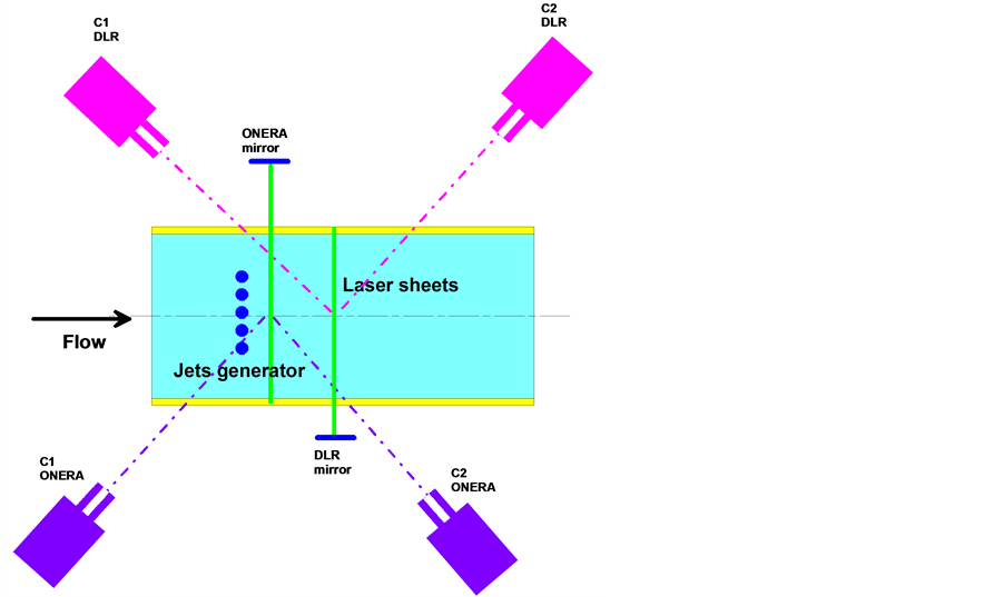
Figure 5. Sketch of the set-up of two 3C-2D-T PIV systems at the test section of the turbulent boundary layer wind tunnel at ONERA, Lille, including the jet actuator row.
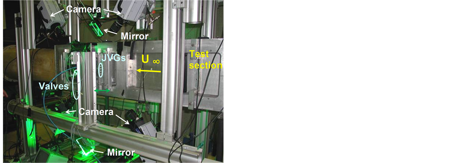
Figure 6. Two synchronized 3C-2D-T PIV systems at the SCL wind tunnel at ONERA, Lille, and support and valves of the (pulsed) jet actuator row. Flow from right to left.
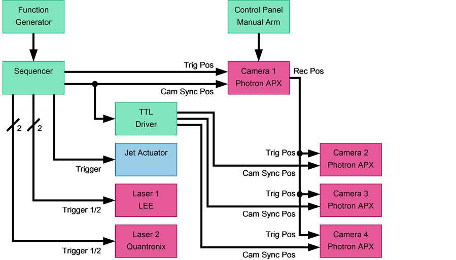
Figure 7. Trigger electronics scheme for synchronization of two high-speed stereo PIV systems and valves of the pulsed jet actuator row.

Figure 8. Timing diagram of the trigger events for synchronization of high-speed cameras and two-laser systems and initiating the valves of the pulsed jet actuator row.
memory on-board have been used. This resulted in a spatial resolution of 1.11 × 1.11 mm2.
Due to a favorable coupling of the image acquisition with the pulse frequency of the jet actuator row (at 50 Hz or 100 Hz) and in order to avoid light pulse interferences of one 3C-2D-T PIV system on the respective images of the other system a camera framing rate of 4 kHz was chosen in order to reach an alternating PIV acquisition frequency of 1 kHz for each system: i.e. both systems acquired double-images at 1 kHz with a phase shift of 500 µsec in between the acquisition of the two high-speed PIV systems.
In order to obtain a proper light-sheet for flow velocity measurements perpendicular to the mean flow, the light beam emitted by each laser passes through a set of spherical and cylindrical lenses. The light-sheets are directed towards the measurement areas through window glass at the test section walls by means of mirrors and had an average thickness of ~2 mm within the fields of view. The DLR system was mounted on a displacement bench to allow an easy translation of the whole optical arrangement between the different measurement planes.
Calibration of both stereo camera systems has been achieved by using a 2 mm thick transparent glass target with regular grid lines printed on one side placed in the respective light-sheet plane and attached to the wall. After mapping of the particle images a disparity correction procedure has been applied in order to correct for the errors in positioning the calibration target and induced by the refractive index changes of the oblique viewing through the glass target from one camera side.
More details about the set-up, in particular a discussion of the timing diagram of the triggering of actuators, lasers, and cameras can be found in [11] [12] . Utilizing the two 3C-2D-T PIV systems it was possible to simultaneously observe the flow velocity field behind the jet generators and in different planes downstream of the actuators simultaneously and in selectable phase relation to the pulsed jets.
As an example for the quality of the results achieved, for  = 30 m/s, a jet pulse frequency of f = 100 Hz and a jet/velocity ratio
  the instantaneous 3-C velocity vector fields at all measured planes at the same phase position of the jet pulse cycle are presented in Figure 9 (z = 0 at middle of five actuator positions). A turbulent boundary layer profile is visible with large coherent areas of u-velocity fluctuations typical for the outer part of the boundary layer above the logarithmic region. The wakes of the pulsed jets are affecting the region below y = 10 mm and are still quite significant at this phase position for the two downstream planes although the velocity fluctuations from the TBL flow is almost of the same amplitude. In the same phase position, the first two planes are already dominated by the passive phase of the jets and the re-organized TBL flow is represented with no direct jet wake interaction. More results and further discussion are provided in [11] [12] .
The cost of the PIV related equipment (two high-speed PIV system requiring high-speed lasers and highspeed cameras) is about 330% of that of a standard (snapshot) 2C-2D PIV system. In order to perform this experiment a man power of about 18 person months was required. The researcher responsible for the PIV experiment should have already carried out several complex PIV measurements, which will require an experience of about 36 person months.
2.3. Three Component-Three Dimensional PIV System with Temporal Resolution (3C-3D-T PIV), Tomographic PIV System
After two decades of development of planar PIV new ideas [13] allowed to address the ultimate goal, i.e. to be able to measure the flow velocity (3C) in a volume (3D) of the flow in a feasible manner and with high accuracy. PIV images of the flow volume taken with several cameras under different observation angles are used to reconstruct the grey level distribution with the tracer particles tomographically. Next, 3D correlation allows determining the instantaneous flow velocity in the observation volume. Intense development work of quite a few research groups allowed to solve most of the problems involved in the use of the new technique (for an overview see [14] ). Today tomographic PIV has been developed far enough to be used in complex applications of fundamental research, including flow control.
As compared with a 3C-2D PIV system tomographic PIV requires at least two additional cameras and Scheimpflug mounts, for the “snap-shot” PIV system as well as for the high-speed PIV system. Also more complex evaluation software for reconstruction of the grey level distribution in the flow volume, 3D cross correlation, and calibration of the multi-camera system is required. PC clusters are used to be able to evaluate the huge amount of data within a reasonable time. As indicated in Figure 1, the size of the observation volume for tomographic PIV is limited due to the limited laser power available and the limited depth of field. For the same observation volume/area the spatial resolution of a 3C-3D PIV system will be less than that of a 3C-2D PIV system.
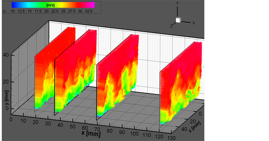
Figure 9. Instantaneous velocity vector fields out of a 1 kHz time series at all investigated planes at U∞ = 30 m/s and 100 Hz jet pulse frequency (measured at the same phase position).
In addition to the capabilities mentioned above a user of a tomographic PIV system should have long-term knowledge and experience in setting up complex illumination and imaging arrangements. Calibration procedures are quite sophisticated. As no immediate on-line evaluation as for 2C-2D or 3C-2D PIV is possible, all steps performed during the measurement (illumination, imaging, recording, calibration etc.) must be done with great care in order to obtain high-quality results. Improvement of the quality of the data after the measurement is usually not possible. In many cases tomographic PIV measurements are carried out in cooperation between research groups due to the costs (and availability) of the required equipment.
Next, the investigation of vortex-generators within a turbulent boundary layer flow shall be taken as example of the application of a 3C-3D-T PIV system [15] . The measurements have been performed together with TU Delft in their water tunnel. The flow generated by an array of vortex-generators (Figure 10), which are located at four different distances (from 106 mm to 1010 mm) upstream of the measurement volume has been observed in a volume of 63 mm × 68 mm × 20 mm using a high-speed Nd:YLF laser at 2 × 25 mJ/pulse at 1 kHz repetition rate and 6 CMOS high-speed cameras (Figure 11). The laser beam is expanded and limited by a rectangular aperture to form a collimated top-hat volume light sheet and enters the water tunnel from above. A flat window in the bottom of a small box immersed in the water surface ensures a smooth transition of the air-water interface. Light is scattered by 56 μm polyamide particles submerged in water. The same tomographic set-up has been used for the investigation of a turbulent boundary layer [16] , where it has been described in detail.
Data is recorded in a time series of 2048 images at 1 kHz making a total observation time of 2 seconds. The final interrogation window size is 323 voxels (corresponding volume 2.7 × 2.7 × 2.7 mm3). The velocity vector data are analyzed as averaged as well as instantaneous data. An example (Figure 12) shows the time-averaged momentum exchange towards the plate being increased (blue) behind the central vortex-generator pair and decreased between the vortex-generator pairs (red). The counter-rotating vortices are visualized by iso-surfaces of vorticity. In the time-resolved results (example Figure 13) the motion and development of flow structures can be analyzed. The contour plot of the (instantaneous) wall-normal velocity is depicted in two selected planes again while flow structures are visualized by iso-surfaces of the swirl (lambda 2). Individual flow structures and their contribution to the flow properties can be identified and can be used as an indicator for flow control efficiency in the device optimization process.
This example shows that tomographic PIV provides the most complete information on the tree-dimensional velocity field of all three PIV systems discussed in this paper. However, as explained before, to operate a tomographic PIV system with optimum performance requires advanced knowledge of the PIV technology as well as
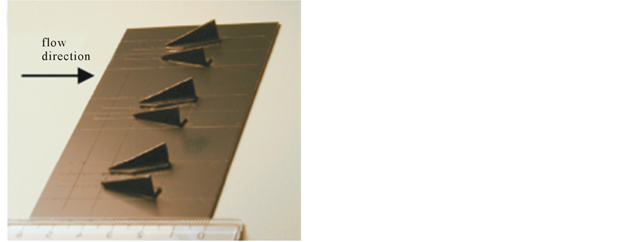
Figure 10. Vortex-generator array.
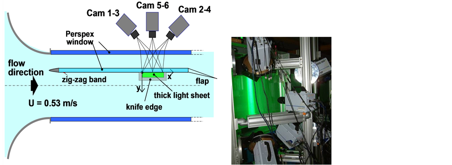
Figure 11. Six CMOS cameras operating at 1 kHz framing rates in a solid angle view at TU Delft water tunnel. The measurement volume of 63 × 15 × 68 mm3 was located in a flat plate TBL flow 2.09 m downstream of the leading edge (see sketch left). Photography of set-up and laser illumination of particles at TU Delft water tunnel (right).
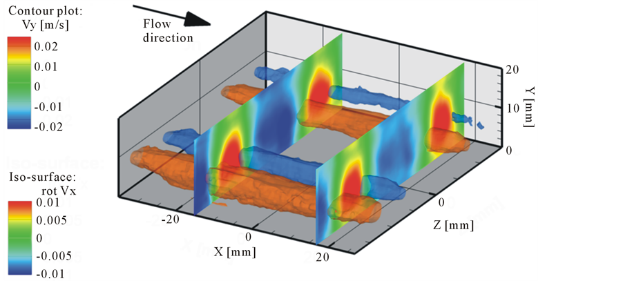
Figure 12. Averaged flow field behind the vortex-generator array.
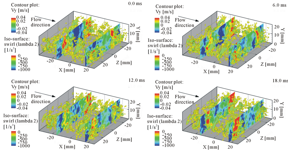
Figure 13. Time-resolved flow field behind the vortex-generator array. Motion and development of the flow structures can be traced from frame to frame (here: 1/6 of actual recording rate for better visibility).
quite a lot of equipment and investment. In order to perform this experiment a man power of about 18 person months was required. The researcher responsible for the PIV experiment should have already carried out several tomographic PIV measurements, which will require an experience of about 48 person months The cost of the PIV related equipment (high-speed PIV system requiring one high-speed laser and six highspeed cameras) is about 400% of that of a standard (snapshot) 2C-2D PIV system.
3. Conclusions
PIV has become an indispensable tool for the investigation of complex unsteady flow fields. For its application to flow control research, different experimental arrangements are available with increasing complexity. The application of tomographic PIV will allow obtaining temporally resolved instantaneous flow fields in a volume of the flow in phase relation to the actuators controlling the flow. The flow control researcher as end user of the PIV technique should select for his investigations that system with the least complexity which will solve his problem. Due to the amount of equipment and experience needed for operation of complex PIV systems cooperation among research groups should be looked for.
One idea for future flow control research work is to use simple and fast PIV systems as sensors for flow control [17] . The use of versatile LED illuminator systems [10] will allow more complex triggering systems for applications where LED light sources are strong enough for illumination.
Also efforts will be made to apply PIV and other image based measurement techniques (PSP (Pressure Sensitive Paint) for measurement of surface pressure, TSP (Temperature Sensitive Paint) for measurement of transition, IPCT (Image Pattern Correlation Technique) for measurement of model surface, MAT (Microphone Array Technique) for measurement of radiated noise etc.) in parallel during the same experiment to obtain a more complete description of the flow field by determining several physical quantities simultaneously for investigation of flow control, transition control, deformation (flutter) control and noise control phenomena.
Acknowledgements
Features and assessment of PIV systems feasible for flow control research, as presented in this paper, are based on the investigations published in references [8] [12] and [15] . We would like to thank all scientists and technicians who contributed to the success of these very complex and demanding investigations. This paper is an update of a keynote paper presented at the 12th International Symposium on Flow Control, Measurement and Visualization (FLUCOME 2013), in Nara, Japan, 2013.
References
- Gad-el-Hak, M. (1996) Modern Developments in Flow Control. Applied Mechanics Review, 49, 365-379. http://dx.doi.org/10.1115/1.3101931
- Aamo, O.M. and Kristic, M. (2003) Flow Control by Feedback: Stabilization and Mixing. Springer, Berlin. http://dx.doi.org/10.1007/978-1-4471-3805-1
- Jahanmiri, M. (2010) Active Flow Control: A Review, Research Report 2010:12. Chalmers University, Gothenburg.
- Raffel, M., Willert, C., Wereley, S. and Kompenhans, J. (2007) Particle Image Velocimetry—A Practical Guide. Springer Verlag, Berlin.
- Adrian, R.J. and Westerweel, J. (2011) Particle Image Velocimetry. Cambridge University Press, Cambridge.
- Stasicki, B., Ehrenfried, K., Dieterle, L., Ludwikowski, K. and Raffel, M. (2001) Advanced Synchronization Techniques for Complex Flow Field Investigations by Means of PIV. 4th International Symposium on Particle Image Velocimetry, Göttingen, 17-19 September 2001, PIV’01 Paper 1188.
- http://www.dlr.de/as/en/desktopdefault.aspx/tabid-183/251_read-12784/
- Ehlers, H., Geisler, R., Gesemann, S. and Schröder, A. (2012) Combined Time-Resolved PIV and Structure Deformation Measurements for Aero-Elastic Investigations. 18. DGLR-Fach-Symposium der STAB, Stuttgart.
- http://www.dlr.de/as/en/desktopdefault.aspx/tabid-183/251_read-13861/
- Stasicki, B., Kompenhans, J., Willert, C. and Ludwikowski, K. (2010) Pulsed LED Illuminator for Visualization, Recording and Measurements of High-Speed Events in Mechanics. Proceedings of the International Conference on Experimental Mechanics (ICEM2010), Kuala Lumpur.
- Gilliot, A., Monnier, J.C., Geiler, C., Delva, J., Schröder, A. and Geisler, R. (2011) Caractérisation par PIV Haute cadence Dual Plane d’une interaction jet/couche limite turbulente. 14iéme Congrès Français de Visualisation et de Traitement d’images en Mécanique des Fluides, Lille.
- Schröder, A., Geisler, R., Schanz, D., Pallek, D., Gilliot, A., Monnier, J.-C., Pruvost, M. and Delva, J. (2012) Effects of Pulsed and Continuous Jet Vortex Generators in a Turbulent Boundary Layer Flow—An Investigation by Using Two High-Speed Stereo PIV Systems. Conference Proceedings of 16th International Symposium on Applications of Laser Techniques to Fluid Mechanics, Lisbon, 9-12 July 2012, 13p. http://ltces.dem.ist.utl.pt/lxlaser/lxlaser2012/upload/362_paper_pnirni.pdf
- Elsinga, G.E., Scarano, F., Wieneke, B. and Van Oudheusden, B.W. (2006) Tomographic Particle Image Velocimetry. Experiments in Fluids, 41, 933-947. http://dx.doi.org/10.1007/s00348-006-0212-z
- Scarano, F. (2013) Tomographic PIV: Principles and Practice. Measurement, Science & Technology, 24, Article ID: 012001. http://dx.doi.org/10.1088/0957-0233/24/1/012001
- Geisler, R., Schröder, A., Willert, C. and Elsinga, G.E. (2008) Investigation of Vortex-Generators within a Turbulent Boundary Layer Flow Using Time-Resolved Tomographic PIV. Conference Proceedings of 14th International Symposium on Applications of Laser Techniques to Fluid Mechanics, Lisbon, 7-10 July 2008, 1p. http://ltces.dem.ist.utl.pt/lxlaser/lxlaser2008/papers/11.1_3.pdf
- Schröder, A., Geisler, R., Staack, K., Henning, A., Wieneke, B., Elsinga, G.E., Scarano, F., Poelma, C. and Westerweel, J. (2010) Eulerian and Lagrangian Insights into a Turbulent Boundary Layer Flow Using Time Resolved Tomographic PIV. New Results in Numerical and Experimental Fluid Mechanics VII Notes on Numerical Fluid Mechanics and Multidisciplinary Design, 112, 307-314.
- Willert, C., Munson, M. and Gharib, M. (2010) Real-Time Particle Image Velocimetry for Closed-Loop Flow Control Applications. Conference Proceedings of 15th International Symposium on Applications of Laser Techniques to Fluid Mechanics, Lisbon, 5-8 July 2010. http://ltces.dem.ist.utl.pt/lxlaser/lxlaser2010/upload/1767_snxsou_1.9.3.Full_1767.pdf