Journal of Flow Control, Measurement & Visualization
Vol.1 No.2(2013), Article ID:34557,12 pages DOI:10.4236/jfcmv.2013.12008
Discrete Tracer Point Method to Evaluate Turbulent Diffusion in Circular Pipe Flow
1Department of Earth Resources Engineering, Faculty of Engineering, Kyushu University, Fukuoka, Japan
2Department of Mining Engineering, Faculty of Mining and Petroleum Engineering, Institut Teknologi Bandung, Bandung, Indonesia
Email: *arifw@mine.kyushu-u.ac.jp
Copyright © 2013 Arif Widiatmojo et al. This is an open access article distributed under the Creative Commons Attribution License, which permits unrestricted use, distribution, and reproduction in any medium, provided the original work is properly cited.
Received February 20, 2013; revised April 10, 2013; accepted May 9, 2013
Keywords: Discrete Tracer Point Method (DTPM); Turbulent Diffusion; Pipe; Numerical Simulation; Airflow
ABSTRACT
Diffusion of a solute in turbulent flows through a circular pipe or tunnel is an important aspect of environmental safety. In this study, the diffusion coefficient of turbulent flow in circular pipe has been simulated by the Discrete Tracer Point Method (DTPM). The DTPM is a Lagrangian numerical method by a number of imaginary point displacement which satisfy turbulent mixing by velocity fluctuations, Reynolds stress, average velocity profile and a turbulent stochastic model. Numerical simulation results of points’ distribution by DTPM have been compared with the analytical solution for turbulent plug-flow. For the case of turbulent circular pipe flow, the appropriate DTPM calculation time step has been investigated using a constant β, which represents the ratio between average mixing lengths over diameter of circular pipe. The evaluated values of diffusion coefficient by DTPM have been found to be in good agreement with Taylor’s analytical equation for turbulent circular pipe flow by giving β = 0.04 to 0.045. Further, history matching of experimental tracer gas measurement through turbulent smooth-straight pipe flow has been presented and the results showed good agreement.
1. Introduction
The diffusion of gas and other particulate matter in pipe or channel flows is important aspect to meet the safety requirements. It controls the longitudinal spreading and the residence time of gases or other particulate matter throughout the pipe. Diffusion occurred in turbulent flow in circular airway has been investigated for a century. Several researches were done by conducting experimental works or numerical approaches. When a pulsed substance or solute is injected into a straight pipe flow, it is advected and diffused to a relative reference moving with certain average velocity. Diffusion in the turbulent pipe flow is mainly characterized by axial velocity profile and velocity fluctuation in flow direction, because the radial gradient of solute concentration is much less than that of flow direction and also radial diffusion is limited by its pipe wall. Furthermore, turbulent mixing motions at different radial positions enhance the diffusion degree in flow direction.
Taylor [1,2] and Aris [3] have made important contributions to develop theories about longitudinal diffusion in pipe flow. Taylor [2] also analyzed longitudinal diffusion in turbulent flow. He used the Reynolds analogy assuming radial diffusivity is analogous with heat and mass transfer in turbulent flow as well as transfer of fluid momentum. He neglected the contribution of molecular diffusion in both radial and axial directions which are negligibly small compared with turbulent eddy mixing diffusion in high Reynolds number. He also evaluated velocity at a certain distance from center of pipe and radial diffusivity as a function of universal velocity profile modified from Goldstein [4]. These assumptions are valid only for higher Reynolds number (Re > 2 × 10⁴) where viscous sublayer and transition layer are negligibly thin. Taylor [2] also proposed the relationship between the longitudinal diffusion coefficient, E (m2/s), against pipe diameter and turbulent shear velocity given by following equations:
 (1)
(1)
 (2)
(2)
where, τ (Pa) and u* (m/s) are shear stress and friction velocity in an arbitrary sub layer of the flow, ρ (kg/m3) is fluid density, d (m) is pipe diameter, f (-) is DarcyWeisbach friction factor and Um (m/s) is cross sectional average velocity.
There are numbers of studies especially for atmospheric pollutant dispersion using random walk as basic method. Most of researches addressed the ideal homogenous turbulence. The pioneer was Taylor [5] who proposed continuous random walk theory for ideal homogeneous turbulent. For his random walk model, Pope [6] applied the well known Langevin equation, a stochastic differential equation. He pointed out the consistency condition in the case of homogeneous turbulent satisfies linear Gaussian model while for inhomogeneous turbulent satisfies non linear Gaussian model. Milojevic [7] simulate particle dispersion in an ideal homogenous flow by incorporating both Lagrangian and Eulerian method. Further, he found high particle concentration at low fluctuation velocity and vice versa. Kroger and Drossinos [8] applied random walk method to simulate thermophoretic particles deposition in turbulent boundary layer using Lagrangian method. He considered velocity, temperature fields and thermophoretic force as Gaussian random fields of which the mean values were obtained from law-to-law wall reactions and from Knudsen number dependent expression of thermophoretic force. The root-mean-square (r.m.s) fluctuation was calculated by polynomial fit with experimental data. Luhar, Ashok and Britter [9] developed random walk for dispersion in a convective boundary layer in inhomogeneous flow. They incorporated well mixed conditions, skewness in vertical velocity and Gaussian random forcing.
Pulsed injection measurement method by using NaCl into water stream in smooth glass pipe was conducted by Sittel, Threadgill and Schnelle [10], while Taylor [2] conducted both in smooth and artificially roughened glass pipes. Furthermore, they applied least square fitting method for their measurements, and showed higher prediction values compared to Taylor’s Equation (1). Higher values of diffusion coefficient were also observed by Hull and Kent [11] by using radioactive tracer injected into a long oil pipelines. Their reason was because of pipe bends and variation in elevation due to terrain profile.
Measurements of diffusion of gas-phase in smooth pipe flows were carried out by Keyes [12], while Davidson, Farqurharson, Picken and Taylor [13] conducted in a rough and long pipeline. Widodo, Sasaki, Gautama and Risono [14] also conducted tracer gas measurement in an underground mine ventilation airways. They found higher diffusion coefficient for the airways flow than those evaluated using Equation (1) for smooth pipe. This phenomenon is well explained by several researchers [15-17]. Compared with obtained data using a solute in water flow, data provided by Keyes [12] and Taylor [2] were measured at relatively lower Reynolds number region. They concluded that the effect of molecular diffusion cannot be neglected in low Reynolds number. Furthermore, because liquid has less molecular transfer, it has a higher Schmidt number compared to gas. Tichacek et al. [17] improved Taylor’s model by considering the molecular diffusion and mean velocity profile based on averaging velocity profiles. They reported that their calculation result deviates significantly for Reynolds number about 4.2 ´ 104, due to the different sets of velocity profile. Thus, the velocity profile used in calculations has a sensitive effect on evaluated values of diffusion coefficient. Figure 1 shows evaluated diffusion coefficients reported in several researches. The empirical relationship proposed by Wen and Fan [18] is also plotted in Figure 1 and shows higher
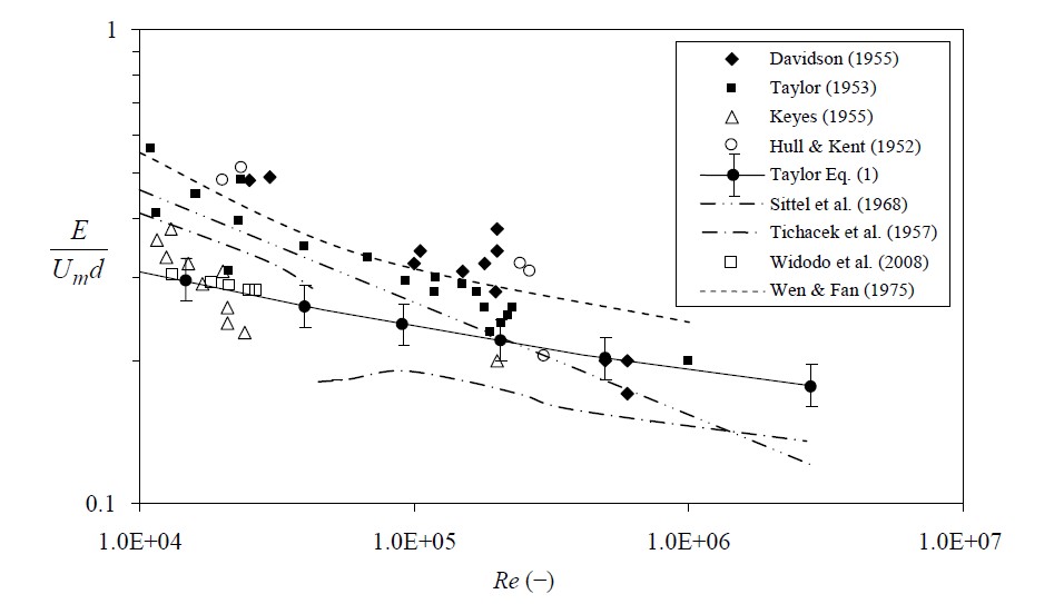
Figure 1. Measurement data, empirical and analytical relationship of longitudinal diffusion coefficient versus Reynolds number from various studies.
prediction compared to [10] and [17]. Taylor’s analytical solution (Equation (1)) is also plotted together with 10% error bars. All have shown the scattered result to each other. Further, it is still necessary to develop further numerical method for gas diffusion in mine airways to simulate the longer travelling time and high diffusion coefficient than those for circular tube flow as demonstrated by Sasaki, Widiatmojo, Arpa and Sugai [19].
The advantages of proposed DTPM are that the calculations of concentration gradient in space or time domain, which are commonly employed in numerical simulations, are not required. It may reduce the computational time. It is also free of grid requirement and the visualization of points’ distribution is simple.
2. Numerical Models Formulations
2.1. Point Movement
The scheme of present numerical simulations has been developed by moving points with regards to velocity profile and turbulent intensities in a turbulent circular pipe flow, depends on radial position of the point in circular cross section. Figure 2 shows schematic variable definitions on the numerical calculation scheme using Cartesian coordinate (x, y, z) to describe tracer positions in circular airway with radius R or diameter d (=2R). The x is distance from the initial position in flow (longitudinal) direction, r is radial position from tube center perpendicular to wall surface, and φ is tangential direction perpendicular to x and r. As for fully developed turbulent flow, mean
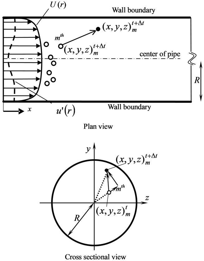
Figure 2. Schematic definition of tracer point movements in pipe flow (x-y and y-z cross sections).
velocities in r and φ directions can be zero.
Turbulent flow is characterized by its stochastic properties. The velocity at a given specific position fluctuates around its mean value. The velocity fluctuation intensity is known as root mean square (r.m.s) values which vary as function of r. The time of averaged flow velocities and the turbulent intensities at a certain position in cylindrical coordinate system (x, r, φ) are defined as (U, 0, 0) and ( ,
,  ,
, ) respectively. The moving of points may be treated easily on Cartesian coordinate system (x, y, z), therefore, in present calculations, turbulent intensities in (x, r, φ) directions are transformed into (x, y, z) directions of Cartesian coordinate. Assumed instantaneous turbulent fluctuations are (
 ,
, ,
, ) in (x, y, z) directions, these can be obtained by transforming velocity fluctuations (
 ,
, ,
, ) as follows (see Figure 3);
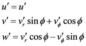 (3)
(3)
Suppose the position of mth point dosed into the flow at origin is denoted with superscript showing the elapsed time, t = 0, its moving distances (Δx, Δy, Δz) during time step Δt are given by;
 (4)
(4)
Its displacement is expressed at t + Δt and t by;
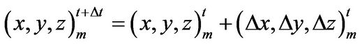 (5)
(5)
Laufer [20] conducted measurements of turbulent intensities and Reynolds stress of air flowing in a straightsmooth pipe with diameter, d = 0.254 m. Measured r.m.s values of turbulent intensities expressed by ( ,
,  ,
, ) in each axis (r, φ, x) were presented as ratios against u* as function of r/R. In present numerical simulations, the polynomial approximations for Laufer’s measurements (see Figure 4) were used to calculate the turbulent intensities at a point’s position, r/R.

Figure 3. Coordinate transformation of velocity vectors in r and φ into y and z direction (Cartesian coordinate).
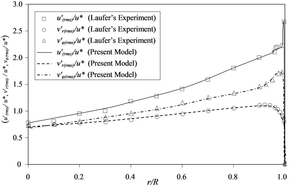
Figure 4. Turbulent model of r.m.s value of turbulent intensities ( ,
,  ,
, ) compared with Laufer’s results.
2.2. Average Velocity Profile
If dimensionless value of longitudinal average velocity is defined as:
 (6)
(6)
Dimensionless distance from the wall is given by:
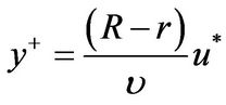 (7)
(7)
where υ (m2/s) is kinematic viscosity. According to Kenyon [21], the relationships of U+ and y+ have been presented by Nikuradse with equations for three regions, that are viscous sub layer (y+ ≤ 5), buffer layer (5 < y+ ≤ 30) and turbulent zone (y+ > 30).
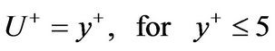 (8)
(8)
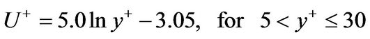 (9)
(9)
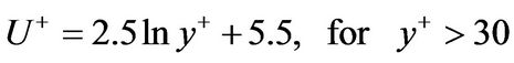 (10)
(10)
Equations (8) to (10) have been confirmed to agree well with equations proposed by Reichardt [22]. In present simulations, these equations were used to calculate axial velocity, U(r) of each point.
2.3. Turbulent Stochastic Model
A stochastic approach was applied to determine points’ diffusion process in the turbulent flow. In present numerical model, it is supposed that the point movements were based on turbulent eddy motion, which satisfies Gaussian probability density function (hereinafter GPDF) with a standard deviation equal to the turbulent intensities or the r.m.s value of velocity fluctuations in each direction (see Rouse [23]). In the simulations, three pseudo-random numbers follow GPDF were generated using Box Muller algorithm to calculate turbulent velocity vector ( ,
,  ,
, ).
).
As described previously, Laufer’s measurement results of turbulent intensities were presented in normalized values over shear velocity, u*, which is function of cross sectional average velocity, Um, and friction factor, f. The relationship between f and Re was presented with empirical equation by Colebrook [24];
 (11)
(11)
2.4. Turbulent Reynolds Stress Model
In turbulent shear flow, fluid particles are translated from slower region to faster one and Reynolds stress is generated. It shows a time-averaged correlation between longitudinal and radial velocity fluctuations in the shear flows. In present study, effects of Reynolds stress correlations have been investigated by giving relationship between x axis velocity fluctuation,  , with velocity fluctuation in r direction,
  , expressed as;
 (12)
(12)
In the simulations, the value of  including its sign was firstly given as a random number following GPDF described previously in preceding chapter, then absolute values of |
 | were generated using similar method, but the signs of u’ were decided to satisfy Equation (12).
2.5. Boundary Condition and Initial Condition
In fact, point’s displacement near wall and its wall interaction has not been well understood to simulate breaking sub-layer. The boundary condition for Lagrangian random walk still needs a calculation model. Several boundary models have been proposed in previous studies. Those methods depend on the physical and numerical factors considered in the simulation [25].
In present DTPM simulations, the reflection boundary condition at the airway wall is satisfied by a repositioning numerical treatment if points are out of the flow region. Thus, by this boundary condition the zero-flux condition at wall can be satisfied. A reflection boundary scheme is modeled as shown in Figure 5 and is used in present simulation. Similar boundary model was also proposed by Szymczak and Ladd [26,27].
Another boundary condition namely rearrangement model has been investigated. In this model, random number is continuously generated until the point is repositioned within the flow regime. Szymczak and Ladd [26] also reviewed this kind of boundary condition as multiple rejection method. Figure 6 shows the comparison of two models. It can be seen that the reflection model resulted in higher dispersion than the rearrangement model. The reason is because the reflection model allows higher possibilities for points to be repositioned at near wall region. These movements make higher “retaining effect” in low velocity layer near wall. Further simulations indicated that the reflection model shows closer results to Taylor’s analytical solution. Thus, reflection model is adapted for present DTPM numerical simulations.
Other zero-flux boundary conditions also have been proposed. Drazer and Koplik [28]; Kurowski, Ippolito,
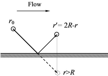
Figure 5. Numerical boundary condition at wall, a reflection model.
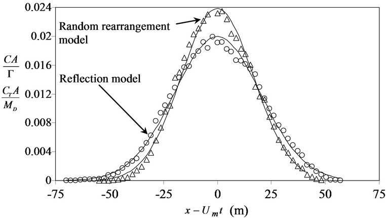
Figure 6. Comparison of numerical result of DTPM after t = 100 s by using different wall boundary conditions (Dt = 0.5 s, Um = 4 m/s, d = 2 m).
Hulin, Koplik and Hinch [29] proposed rejection boundary where the points do not change its position in the given time step and other random diffusivity is recalculated until the movement satisfy r < R. Salles et al. [30] and Maier et al. [31] suggested interruption boundary condition at which points stop at wall and its time is incremented by modified time step, λDt where λ = 0 ~ 1 is adjustment factor. However, only the reflection method imposes the zero-flux boundary condition while other boundary conditions lead to incorrect concentration profiles near wall boundary [26].
3. Calculation Results and Evaluation of Diffusion Coefficient
3.1. One-Dimensional Diffusion
Taylor [1,2] proposed that concentration distribution of solute after certain time, t, is symmetrically distributed follows the partial differential equation. He proposed concentration gradient at x and r direction which move to x direction with constant average cross sectional velocity, Um;
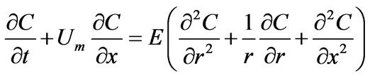 (13)
(13)
Several studies (see Wen and Fan [18]) also proposed similar numerical expression of solute diffusion plug flow model.
The solution of Equation (13) can be obtained by assuming that molecular diffusion is neglected and concentration gradient in radial direction is negligible. The variable, E shows effective diffusion coefficient in axial direction. Since the center of dispersed solute is assumed to be at x = Umt after elapsed time, t, the solution of Equation (13) can be given with an equation similar with Gaussian distribution:
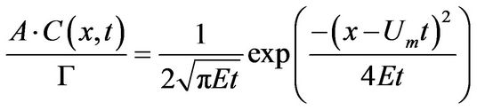 (14)
(14)
where G (m3) is total volume of released solute at x = 0, and A (m2) is cross sectional area of pipe.
In the DTPM simulation, concentration of diffused points, C, can be calculated by;
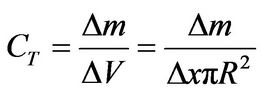 (15)
(15)
where Δm is number of point counted in the numerical control volume which located at a certain downstream position, given by ΔV = ΔXπd2/4 and ΔX = UmΔt. Suppose the total number of points released from the origin is MD, The normalized concentration of points is expressed as CTA/MD.
3.2. Simulation of Turbulent Flow through Circular Airway
The DTPM simulations on turbulent flow of a straightsmooth airway have been carried out. Figure 7 shows the evolution of point’s distribution after several elapsed time since released into the flow (Um = 1.5 m/s, d = 0.5 m). It can be observed that the asymmetry of points distribution is gradually diminished as the travelled distance increases.
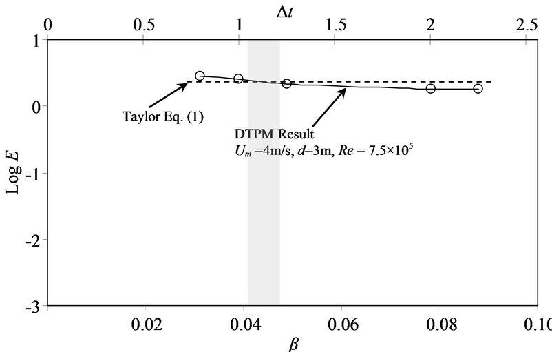
Figures 8 and 9 show the results of simulation for flow with d = 2 m, Um = 4 m/s (f = 0.01315) and d = 4 m, Um = 5 m/s (f = 0.0112) respectively after t = 100 s. It can be inferred that different calculation time step, Δt, gives different evaluated value of effective diffusion coefficient. To consider this effect, the evaluated value of effective diffusion coefficient is plotted against dimensionless value, β (-) defined as:
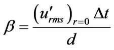 (16)
(16)
where  is r.m.s value of streamwise velocity fluctuation in the center of pipe. It may be possible to
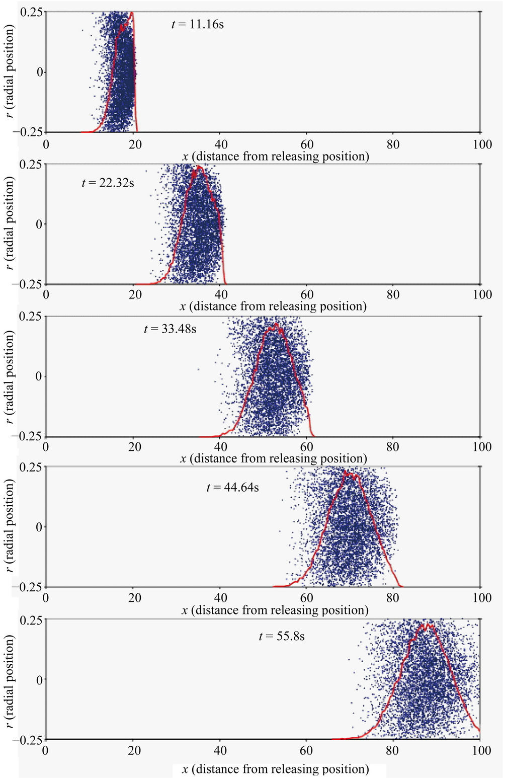
Figure 7. Points distribution showing diffusion in longitudinal direction for Um = 1.5 m/s, d = 0.5 m, ∆t = 1 s, f = 0.0211, after five consecutive elapsed time (horizontal axis and vertical axis is travelled distance in flow direction and radial distribution respectively).
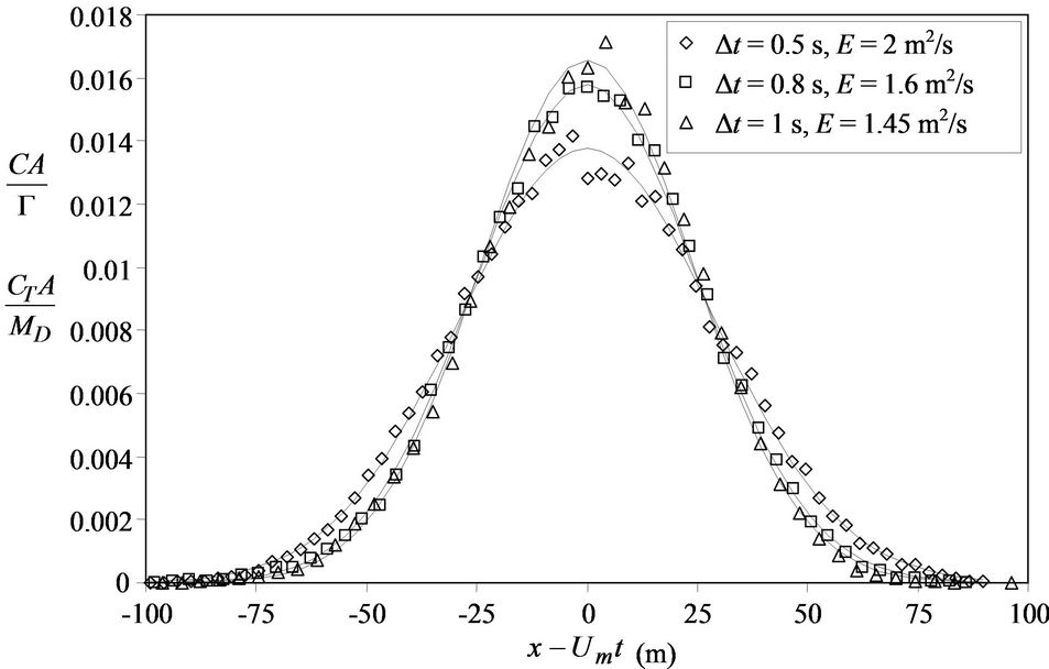
Figure 8. Results of DTPM simulation with different Δt at t = 200 s for circular channel flow with Um = 4 m/s, d = 2 m (f = 0.01315).
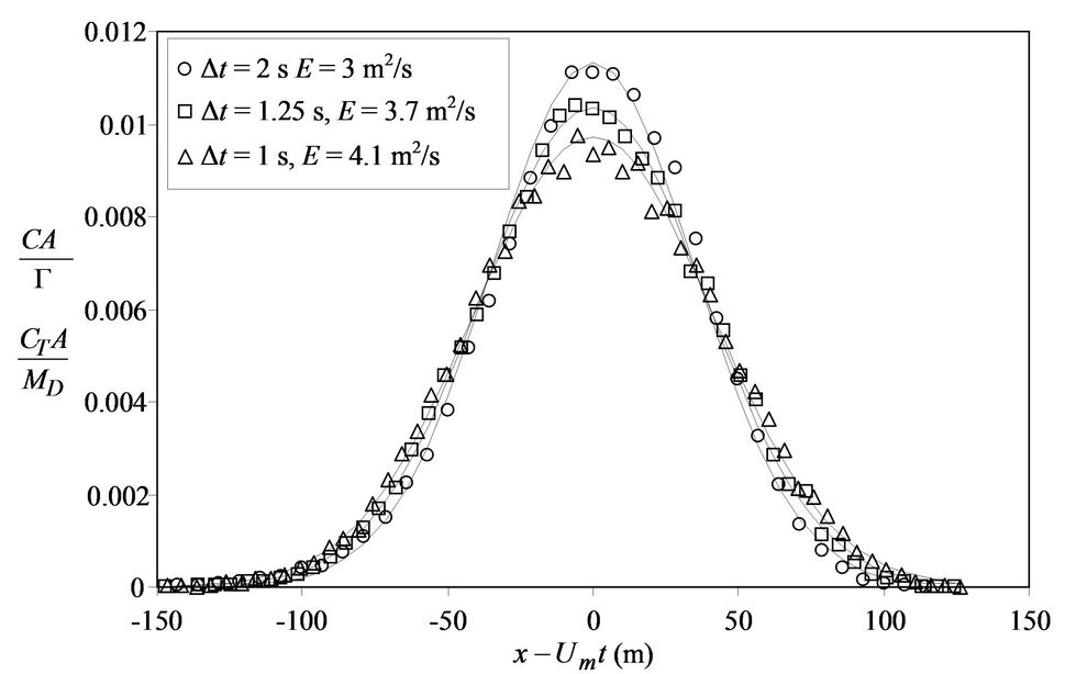
Figure 9. Results of DTPM simulation with different Δt at t = 200 s for circular channel flow with Um = 5 m/s, d = 4 m (f = 0.0112).
regard β as ratio of the average mixing length to pipe diameter.
Figures 10(a)-(d) shows evaluated values of effective diffusion coefficient of different time step for Re = 5 × 10⁵, 7.5 × 10⁵, 9.4 × 10⁵ and 1.25 × 10⁶. The values of E calculated by Equation (1) are also presented as comparisons. From the results, it can be seen that the evaluated values of E from present DTPM for β = 0.04 ~ 0.045 intersect with those Taylor analytical solution given by Equation (1).
The results of evaluated E of DTPM showing relatively non-linear and inversely proportional correlation to the value of β, before gradually attain constant value as higher value of Δt is applied. Further simulations were done by setting β = 0.040, 0.043 and 0.045 at different flow conditions. As shown in Figure 11, the results indicate linear relationship between Taylor’s analytical equation and ones evaluated by DTPM. The value of β = 0.043 used for DTPM simulations is appropriate in order to get longitudinal diffusion coefficient, E, which has good agreement with Taylor’s analytical solution.
4. Simulation of Tracer Gas Experiment through Smooth-Circular Pip
Tracer gas diffusion experiment was conducted at a laboratory scale by Widodo [32]. The experimental apparatus mainly consists of smooth circular pipe as scaled pipe, gas injection apparatus, and gas measurement apparatus.
For the straight airway, he used a pipe with smooth lining 0.025 m diameter, 30 m length and placed horizontally. Tracer gas was released by breaking balloons filled with methane (CH4) and measured arriving concentration at the end of pipe. Methane concentration was measured by an original infrared adsorption gas detector
 (a)
(a) (b)
(b)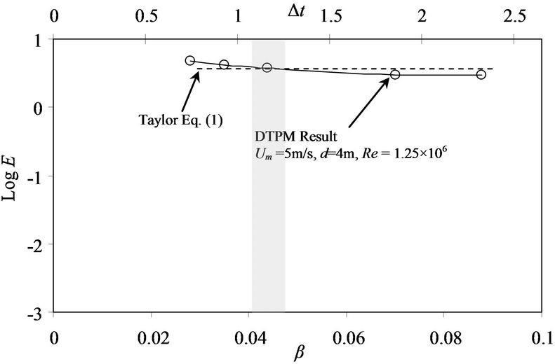 (c)
(c)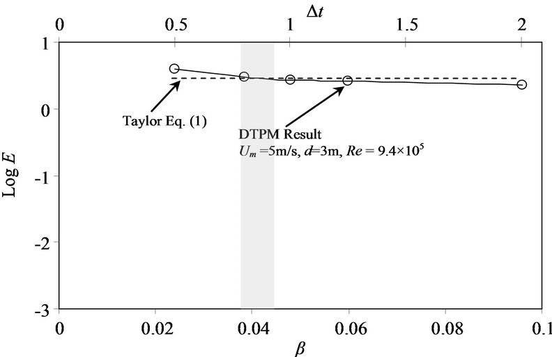 (d)
(d)
Figure 10. Effect of dimensionless value, β, on evaluated diffusion coefficient, E, for different Reynolds number compared with Taylor’s analytical solution given by Equation (1). (a) Re = 5 × 10⁵; (b) Re = 7.5 × 10⁵; (c) Re = 9.4 × 10⁵; (d) Re = 1.25 × 10⁶.
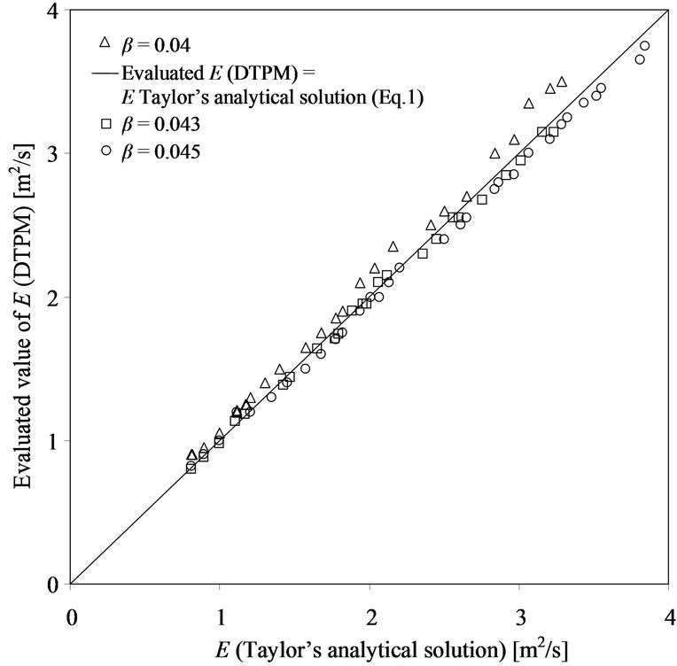
Figure 11. Evaluated result of diffusion coefficient evaluated by DTPM considering β = 0.04, 0.043 and 0.045 compared with Taylor solution of (Equation (1)).
using 3.4 mm He-Ne laser with an infrared (IR) sensor, air pump, air mass flow meter and amplifier as shown in Figure 12. Sampling rate was set as the maximum flow rate at which the gas sensor could still detect the gas concentration correctly. The data were recorded with a data logger connected to a PC.
Beforehand, the conversion of voltage reading by data logger to gas concentration was calibrated based on calibration data with the standard methane-air mixture. The validity of concentration reading from IR sensor was crosschecked using gas chromatograph and showed good linear fit.
The measurement was conducted for Reynolds number, Re = 6085 (Um = 3.87 m/s, d = 2R = 0.025 m). Measurements for higher Re were also done; however, the data were inadequately acquired due to insufficient sampling rate to compensate higher flow velocity.
For the DTPM simulation, calculation parameters were decided based on the experimental properties such as pipe’s length, average cross sectional velocity and pipe’s diameter. Value of friction factor, f, was calculated using Equation (11) and calculation time step was defined using Equation (16) as Dt = 0.0092 s. To verify the effect of initial points’ distribution, three different conditions were considered; 1) point source (x0 = 0, r0 = 0); 2) uniformly distributed at x0 = 0 (0 ≤ r0 < R); 3) uniformly distributed at x0 ± 2d.
Figure 13 shows the evolution of radial and longitudinal point’s distribution in five consecutive times for point source initial condition. The results shown in Figure 14 implied that the difference of initial points’ distribution has no significant effect on result of DTPM. The length of flow domain is long enough for the radial diffusivity to attain radial homogeneity of flow. It may also imply that the sudden break of balloons during release has less effect on the arriving concentration as the measurement distance is long compared to diameter d![]() pipe length. In general, the results confirm that present DTPM is able to simulate the turbulent in straight and smooth circular pipe.
pipe length. In general, the results confirm that present DTPM is able to simulate the turbulent in straight and smooth circular pipe.
In the real case, the utilization of tracer gas measurement is not merely straight pipe, but also tunnels network [19,32-35]. This kind of network is assembled in the form of interconnecting tunnels which allow airflow to be separated or rejoined at junction. The mechanism of points tracking as proposed in this study can be developed to consider network flow by combining with a scheme to treat flow separation. The developed scheme is supposed to be able to simulate point’s distribution at arbitrary position in the network and allow easy dispersion evaluation of gas or other particulates spreading.
5. Conclusions
In this study, effective diffusion coefficients of turbulent flow in circular pipe or channel have been evaluated by the Discrete Tracer Point Method (DTPM), a Lagrangian numerical simulation method. The present study is summarized as follows:
1) DTPM simulation procedures have been presented to
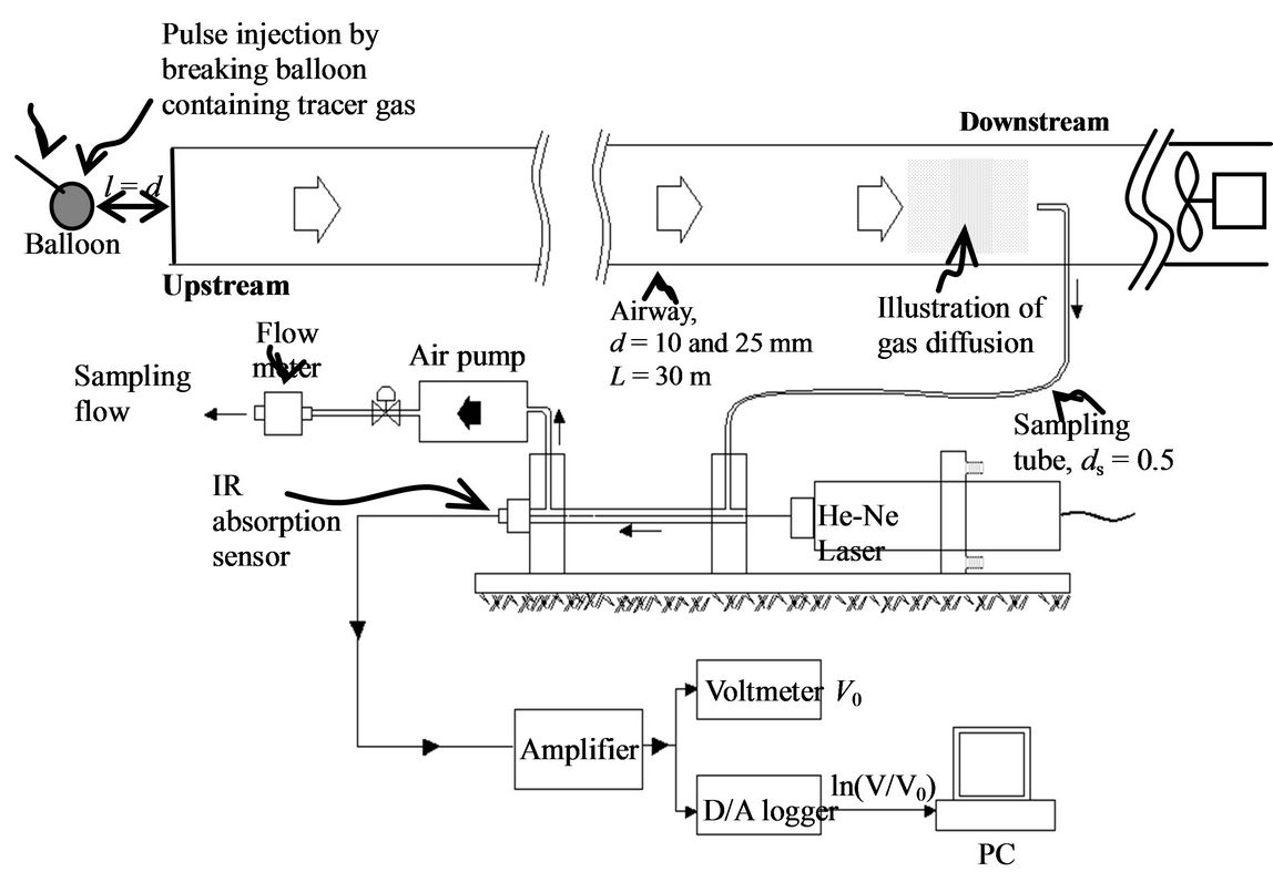
Figure 12. Experimental setting for turbulent diffusion through circular smooth-straight pipe (after Widodo [32]).
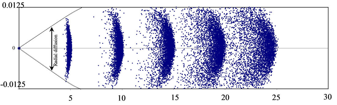
Figure 13. Point distribution after t = 1.08 s, t = 2.16 s, t = 3.24 s, t = 4.32 s, t = 5.40 s with point source initial condition; (Um = 3.87 m/s, d = 0.025 m, ∆t = 0.0092 s, f = 0.0211, horizontal axis and vertical axis is travelled distance in flow direction and radial distribution respectively).
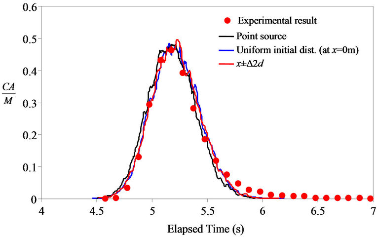
Figure 14. Simulation results with different initial condition of points distribution for Um = 3.87, d = 0.025 m, f = 0.035.
simulate the displacement of points released into straightsmooth circular airway flow by giving turbulent average velocity, intensity of velocity fluctuation and Reynolds stress;
2) A simple procedure to represent diffusion of points in the airway flow has been employed by generating random number which satisfies Gaussian probability functions with value of turbulent intensities in each direction as standard deviations;
3) Appropriate calculation time step was proposed by matching with Taylor’s analytical equation by considering the ratio between the average mixing lengths to airway’s diameter, β @ 0.043;
4) The result of matching curve of DTPM with experimental result by considering different initial points distribution has shown that the present DTPM can be used to simulate turbulent advection-diffusion in smoothstraight pipe representing the ideal model of straight pipe or channel;
5) Present DTPM simulation has promising possibility to simulate the network flow by combining with a scheme to treat flow separation at junction.
6. Acknowledgements
Authors would like to thank Japan Ministry of Education, Culture, Sports, Science and Technology and Kyushu University Global COE program for the financial support.
REFERENCES
- G. I. Taylor, “Dispersion of Soluble Matter in Solvent Flowing Slowly through a Tube,” Proceedings of the Royal Society of London. Series A. Mathematical and Physical Sciences, Vol. 219, No. 1137, 1953, pp. 186-203. doi:10.1098/rspa.1953.0139
- G. I. Taylor, “The Dispersion of Matter in Turbulent Flow through a Pipe,” Proceedings of the Royal Society of London. Series A. Mathematical and Physical Sciences, Vol. 223, No. 1155, 1954, pp. 446-468. doi:10.1098/rspa.1954.0130
- R. Aris, “On the Dispersion of a Solute in a Fluid Flowing through a Tube,” Proceedings of the Royal Society of London. Series A. Mathematical and Physical Sciences, Vol. 235, No. 1200, 1956, pp. 67-77. doi:10.1098/rspa.1956.0065
- S. Goldstein, “Modern Developments in Fluid Dynamics,” Dover, New York, 1965.
- G. I. Taylor, “Diffusion by Continuous Movements,” Proceedings of London Mathematical Society, Vol. 20, No. 1, 1954, pp. 196-211. doi:10.1112/plms/s2-20.1.196
- S. B. Pope, “Consistency Conditions for Random-Walk Models of Turbulent Dispersion,” Physics of Fluids, Vol. 30, No. 8, 1987, pp. 2374-2379. doi:10.1063/1.866127
- D. Milojevic, “Lagrangian Stochastic-Deterministic Predictions of Particle Dispersion in Turbulence,” Particle & Particle Systems Characterization, Vol. 7, No. 1-4, 1990, pp. 181-190. doi:10.1002/ppsc.19900070132
- C. Kröger and Y. Drossinos, “A Random-Walk Simulation of Thermophoretic Particle Deposition in a Turbulent Boundary Layer,” International Journal of Multiphase Flow, Vol. 26, No. 8, 2000, pp. 1325-1350. doi:10.1016/S0301-9322(99)00092-0
- A. K. Luhar and R. E. Britter, “A Random Walk Model for Dispersion in Inhomogeneous Turbulence in a Convective Boundary Layer,” Atmospheric Environment, Vol. 23, No. 9, 1989, pp. 1911-1924. doi:10.1016/0004-6981(89)90516-7
- C. N. Sittel Jr., W. D. Threadgill and K. B. Schnelle Jr., “Longitudinal Dispersion for Turbulent Flow in Pipes,” Industrial & Engineering Chemistry Fundamentals, Vol. 7, No. 1, 1968, pp. 39-43. doi:10.1021/i160025a007
- D. E. Hull and J. W. Kent, “Radioactive Tracers to Mark Interfaces and Measure Intermixing in Pipelines,” Industrial & Engineering Chemistry, Vol. 44, No. 11, 1952, pp. 2745-2750. doi:10.1021/ie50515a066
- J. J. Keyes Jr., “Diffusional Film Characteristics in Turbulent Flow: Dynamic Response Metho,” AiChE Journal, Vol. 1, No. 3, 1955, pp. 305-311. doi:10.1002/aic.690010306
- F. Davidson, D. C. Farqurharson, J. Q. Picken and D. C. Taylor, “Gas Mixing in Long Pipelines,” Chemical Engineering Science, Vol. 4, No. 5, 1955, pp. 201-205. doi:10.1016/0009-2509(55)80006-1
- N. P. Widodo, K. R. Sasaki, R. S. Gautama and Risono, “Mine Ventilation Measurements with Tracer Gas Method and Evaluations of Turbulent Diffusion Coefficient,” International Journal of Mining, Reclamation and Environment, Vol. 22, No. 1, 2008, pp. 60-69. doi:10.1080/17480930701474869
- W. B. Krantz and D. T. Wasan, “Axial Dispersion in the Turbulent Flow of Power-Law Fluids in Straight Tubes,” Industrial & Engineering Chemistry Fundamentals, Vol. 13, No. 1, 1974, pp. 56-62. doi:10.1021/i160049a011
- O. Levenspiel, “Longitudinal Mixing of Fluids Flowing in Circular Pipes,” Industrial & Engineering Chemistry, Vol. 50, No. 3, 1958, pp. 343-346. doi:10.1021/ie50579a034
- L. J. Tichacek, C. H. Barkelew and T. Baron “Axial Mixing in Pipes,” AIChE Journal, Vol. 3, No. 4, 1957, pp. 439- 442. doi:10.1002/aic.690030404
- C. Y. Wen and L. T. Fan, “Models for Flow System and Chemical Reactors,” Dekker, New York, 1975.
- K. Sasaki, A. Widiatmojo, G. Arpa and Y. Sugai, “Airflow Measurements and Evaluation of Effective Diffusion Coefficient in Large Scale of Mine Ventilation Network Using with Tracer Gas Method,” Journal of the Mining and Materials Processing Institute of Japan, Vol. 125, No. 12, 2009, pp. 614-620. doi:10.2473/journalofmmij.125.614
- J. Laufer, “The Structure of Turbulent in Fully Developed Pipe Flow,” Technical Report 1174, National Committee for Aeronautics, 1954. http://naca.central.cranfield.ac.uk/report.php?NID=5843
- R. A. Kenyon, “Principles of Fluid Mechanics,” Ronald Press, New York, 1960.
- H. Reichardt, “Complete Representation of the Turbulent Velocity Distribution in Smooth Pipes,” Journal of Applied Mathematics and Mechanics, Vol. 31. No. 7, 1951, pp. 208-219. doi:10.1002/zamm.19510310704
- H. Rouse, “Advanced Mechanics of Fluids,” John Wiley and Sons, Inc., New York, 1959.
- C. F. Colebrook, “Turbulent Flow in Pipes, with Particular Reference to the Transition Region between the Smooth and Rough Pipe Laws,” Journal of the ICE, Vol. 11, No. 4, 1939, pp. 133-156. doi:10.1680/ijoti.1939.13150
- D. J. Thomson, W. L. Physick and R. H. Maryon, “Treatment of Interfaces in Random Walk Dispersion Models,” Journal of Applied Meteorology, Vol. 36, No. 9, 1997, pp. 1284-1285. doi:10.1175/1520-0450(1997)036<1284:TOIIRW>2.0.CO;2
- P. Szymczak and A. J. C. Ladd, “Boundary Conditions for Stochastic Solutions of the Convection-Diffusion Equation,” Physical Review E, Vol. 68, No. 3, 2003, Article ID: 036704. doi:10.1103/PhysRevE.68.036704
- P. Szymczak and A. J. C. Ladd, “Stochastic Boundary Conditions to the Convection-Diffusion Equation including Chemical Reactions at Solid Surfaces,” Physical Review E, Vol. 69, No. 3, 2004, Article ID: 036704. doi:10.1103/PhysRevE.69.036704
- G. Drazer and J. Koplik, “Tracer Dispersion in Two-Dimensional Rough Fractures,” Physical Review E, Vol. 63, No. 5, 2001, Article ID: 056104. doi:10.1103/PhysRevE.63.056104
- P. Kurowski, I. Ippolito, J. P. Hulin, J. Koplik and E. J. Hinch, “Anomalous Dispersion in a Dipole Flow Geometry,” Physics of Fluids, Vol. 6, No. 1, 1994, pp. 108-117. doi:10.1063/1.868075
- J. Salles, J. F. Thovert, R. Delannay, L. Prevors, J.-L. Auriault and P. M. Adler, “Taylor Dispersion in Porous Media. Determination of the Dispersion Tensor,” Physics of Fluids A: Fluid Dynamics, Vol. 5, No. 10, 1993, pp. 2348-2376. doi:10.1063/1.858751
- R. S. Maier, D. M. Kroll, R. S. Bernard, S. E. Howington, J. F. Peters and H. T Davis, “Pore-Scale Simulation of Dispersion,” Physics of Fluids, Vol. 12, No. 8, 2000, pp. 2065-2079. doi:10.1063/1.870452
- N. P. Widodo, “Study on Tracer Gas Method for Mine Ventilation Measurement and Evaluation of Gas Diffusion Coefficient,” Ph.D. Thesis, Kyushu University, Fukuoka, 2008.
- G. Xu, K. D. Luxbacher, S. Ragab and S. Schafrik, “Development of a Remote Analysis Method for Underground Ventilation Systems Using Tracer Gas and CFD in a Simplified Laboratory Apparatus,” Tunneling and Underground Space Technology, Vol. 33, 2013, pp. 1-11. doi:10.1016/j.tust.2012.09.001
- M. H. Johnson, Z. Zhai and M. Krarti, “Performance Evaluation of Network Airflow Models for Natural Ventilation,” HVAC&R Research, Vol. 18, No. 3, 2012, pp. 349-365.
- R. Gao, A. Li, X. Hao, W. Lei and B. Deng, “Prediction of the Spread of Smoke in a Huge Transit Terminal Subway Station under Six Different Fire Scenarios,” Tunnelling and Underground Space Technology, Vol. 21, 2012, pp. 128-138. doi:10.1016/j.tust.2012.04.013
Nomenclature
A = Cross-sectional area of pipe (m2)
C = Gas concentration (−)
CT = Number of points located within numerical control volume (−)
d = Diameter of pipe (m)
E = Longitudinal diffusion coefficient (m2/s)
f = Darcy-Weisbach friction factor (−)
MD = Total number of released points (−)
r = Radial position of a point (m)
R = Radius of pipe (m)
Re = Reynolds number (−)
t = Elapsed time (s)
U = Time-averaged flow velocity in x direction u* = Friction velocity (m/s)
U+ = Dimensionless value of flow velocity (−)
y+ = Dimensionless distance from the wall (−)
Um = Cross-sectional average velocity (m/s)
( ) = Turbulent intensities in cartesian coordinate (x, y, z) (m/s)
 = Stream-wise velocity fluctuation in the pipe center (m/s)
( ,
, ,
, ) = Turbulent intensities in cylindrical coordinate (r, φ, x) (m/s)
( ,
,  ,
, ) = r.m.s value of turbulent intensities in cylindrical coordinate (r, φ, x) (m/s)
(Δx, Δy, Δz) = Displacement vector of a point (m)
β = ratio between average mixing in stream-wise direction to the diameter of pipe
Γ = Released volume of tracer gas (m3)
Δt = Numerical time step (s)
ΔV = Numerical control volume (m3)
λ = Time adjustment factor for interruption boundary condition (−)
ρ = Density of fluid (kg/m3)
τ = Shear stress (Pa)
υ = Kinematic viscosity of fluid (m2/s)
NOTES
*Corresponding author.