Journal of Flow Control, Measurement & Visualization
Vol. 1 No. 1 (2013) , Article ID: 30577 , 7 pages DOI:10.4236/jfcmv.2013.11003
Wake-Induced Bypass Transition over a Flat Plate under Favorable and Adverse Pressure Gradients
1Department of Mechanical Engineering, Tomakomai National College of Technology, Tomakomai, Japan
2Department of Engineering and Applied Sciences, Sophia University, Tokyo, Japan
Email: e-koyabu@me.tomakomai-ct.ac.jp
Copyright © 2013 Eitaro Koyabu, Tetsuhiro Tsukiji. This is an open access article distributed under the Creative Commons Attribution License, which permits unrestricted use, distribution, and reproduction in any medium, provided the original work is properly cited.
Received December 20, 2012; revised February 5, 2013; accepted February 18, 2013
Keywords: Boundary Layer; Wake; Transition; Pressure Gradient; Hot-Wire Anemometry
ABSTRACT
The present study investigates wake-induced bypass transition of boundary layers on a flat plate subjected to favorable and adverse pressure gradients. The aim is to exploit unsteady effects in order to design an aft-loaded turbine blade without increasing the profile loss, as has been achieved for low pressure turbine blades. First of all, this fundamental study is to reveal the effect of the Strouhal number, which changed by using different numbers of wake generating bars. Detailed boundary layer measurements were conducted using two hot-wire probes. A passage-contouring device was employed to generate a pressure gradient on the test model, which was typical to that generated by an aft-loaded turbine blade. A spoked-wheel-type wake generator was used to create periodic wakes in front of the flat plate. It was found that the wake passage induces a significant change in the flow structure downstream of the flow acceleration region.
1. Introduction
The flow field in turbomachines is characterized by complicated flow that has three dimensional effects from unsteady flow. Recently, owing to the demand for higher gas turbine efficiency, there is an increased need to better understand unsteady effects on the aerodynamics, heat transfer, and noise in turbomachinery. Many researchers have been studying the transition process of the boundary layer on turbomachinery blades in a flow that is periodically disturbed by the rotor wakes [1-8]. It is essential to quantitatively predict these effects at the design stage. However, the effect of the unsteady flow on boundary layer transition is not fully understood. Bypass transition is defined as the direct production of turbulent spots in the boundary layer by high free-stream turbulence levels [1]. That is, the initial two-dimensional instability phase of a natural transition is bypassed in this case. A natural transition is a classical process that arises from the appearance of the two-dimensional Tollmien-Schlichting instability waves in the laminar boundary layer. With that in mind, this study investigates the effect of the Strouhal number of wake on the transition onset of the boundary layer on a flat plate, which is subjected to favorable and adverse pressure gradients. Detailed boundary layer measurements are performed by hot-wire anemometry. A passage-contouring device similar to that used by Ottavy et al. [9] was employed to generate a pressure gradient on the test model, which was typical to that generated by an aft-loaded turbine blade. A spoked-wheel-type wake generator is used to simulate the unsteady flow field over the suction surface of a turbine rotor.
2. Experimental Setup
The wind tunnel is closed-circuit wind tunnel. Figure 1 shows the schematic of the test apparatus used in this study: two honeycombs set in the settling chamber. The cross-section area of each honeycomb is 1030 × 1030 mm and the diagonal size of honeycomb is about 10 mm. The settling chamber and the contraction nozzle reduced the free-stream turbulence to approximately 2% [10]. Periodic wakes were produced by a spoked-wheel-type generator that consisted of a disk of 300 mm diameter and cylindrical bars of 10 mm diameter. The revolution number of the disk in the wake generator was counted by an optical tachometer. The fluctuation in revolution was observed to be less than 0.5%. The rotation direction of the disk in the wake generator was the movement of the wake generating bar relative to the test model in
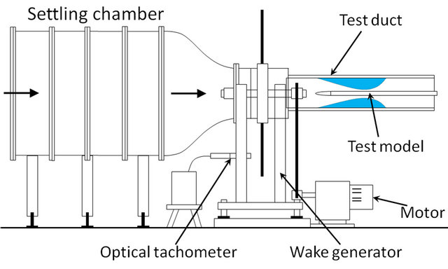
Figure 1. Test apparatus.
Figure 2. The flow field corresponds to the interaction between the wake and boundary layer over the suction surface. This fluid motion is the so-called “negative jet”, which seemed to have some effects on the transitional behavior of the wake-disturbed boundary layer. Figure 2 shows the test model, the wake generator and passagecontouring devices attached on the top and bottom walls of the test duct. The wake generator was set so that each of the wake-generating bars became parallel with the leading edge of the test model when it moved in front of the model. A 0.6 m long test model made of acrylic resin plates was used. It had a semi-elliptic leading edge with a long axis of 75 mm and a short axis of 15 mm, followed by a flat-plate afterbody. The width and thickness were 200 and 30 mm, respectively. Static pressure taps were provided on one side of the test model to measure the pressure distribution on the test surface. The passagecontouring devices were shaved from styrofoam bricks so as to assume a shape for establishing a pressure gradient typical to that generated by an aft-loaded turbine blade. Figure 2 also shows the system for the boundary layer measurement based on hot-wire anemometry. The passage-contouring device had two slots for inserting the hot-wire probes into the main flow. Both slots were securely plugged with several blocks to prevent the leakage from the slot.
3. Instrumentation and Data Processing
3.1. Ensemble-Averaged Quantities
Two hot-wire probes used to measure the boundary layer on the test model were placed at the measurement location to a precision of ±0.01 mm by a PC-controlled traversing unit. They were connected to a constant-temperature anemometer. By monitoring the free-stream temperature at the exit of the test section, the temperature unit effectively compensated for the temperature fluctuation of relatively low frequency, during a long-running measurement. The linearized signals from the probes were acquired and digitized by an A/D converter using a once-per-revolution signal from the optical tachometer as
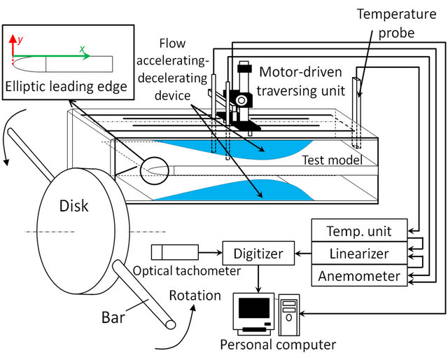
Figure 2. Test model and the system for boundary layer measurement.
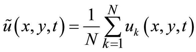
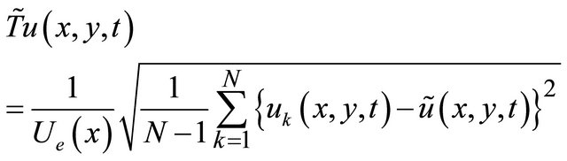
the synchronization signal, which guaranteed the application of the phase-locked averaging technique to the sample data. The data-sampling rate was 20 kHz, and each of the digitized records contained 2500 words. The phase-locked or ensemble-averaged velocity,  , was then calculated from the acquired instantaneous velocity data, uk (k = 1, 2, ···, 100; N = 100) as per the following equation:
 (1)
(1)
where x, y, t, and N are the longitudinal distance from the leading edge, distance from the surface of the test model, time, and number of sampled data, respectively. The ensemble-averaged turbulence intensity  is also defined by
 (2)
(2)
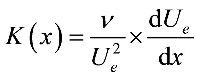
where Ue(x) was the local velocity determined from the static pressure measurements with the Bernoulli’s equation.
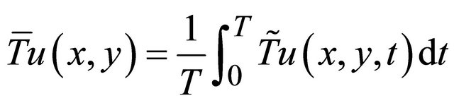
3.2. Time-Averaged Quantities
Time-averaged quantities were obtained by the integrating the ensemble-averaged quantities over the wakepassing period. For instance, the time-averaged turbulence intensity  was calculated by
 (3)
(3)
where T is the wake-passing period.
3.3. Uncertainty
Uncertainties of the inlet velocity and instantaneous velocity were respectively estimated to be about 2% and 3% using the Kline and McClintock method [11].
3.4. Test Conditions
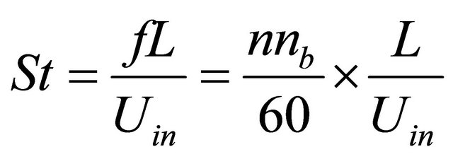
Wake-disturbed unsteady flow field around the test model was characterized by two non-dimensional numbers, namely, Reynolds number Re, and Strouhal number St which are respectively defined as:
 (4)
(4)
 (5)
(5)
where Uin is inlet velocity, L is the length of the test model,  is wake-passing frequency and
 ![]() is kinematic viscosity. Table 1 shows the test conditions in this study. Test Case 1 was a baseline experiment with no wake, where the inlet velocity Uin was 6.2 m/s and the Reynolds number Re based on the length of the test model and the inlet velocity was 2.5 × 10⁵. The Strouhal number was 0.97, 1.94, and 2.90, when the bar count nb was 2, 4, and 6, respectively; f is the wake frequency; the disk rotational speed n was 300 rpm; and the length of the test model L was 0.6 m. The application of this study is the low-pressure turbine. For real machines, the range of the Strouhal number is from 0.3 to 1.2 [7,8], and in this study it is from 0.97 to 2.90. To specially investigate the effect of the Strouhal number on the transition of the boundary layer, we chose a range of the Strouhal number slightly larger than that of the real machine. The horizontal distances between the center of the disk of the wake generator and the extended lines of the slots of probe 1 and probe 2 were 265 and 365 mm, respectively. Therefore, the moving speeds of the bar on the extended lines of the slots of probe 1 and probe 2 were 8.3 and 12.4 m/s, respectively. The measurement region extended from
is kinematic viscosity. Table 1 shows the test conditions in this study. Test Case 1 was a baseline experiment with no wake, where the inlet velocity Uin was 6.2 m/s and the Reynolds number Re based on the length of the test model and the inlet velocity was 2.5 × 10⁵. The Strouhal number was 0.97, 1.94, and 2.90, when the bar count nb was 2, 4, and 6, respectively; f is the wake frequency; the disk rotational speed n was 300 rpm; and the length of the test model L was 0.6 m. The application of this study is the low-pressure turbine. For real machines, the range of the Strouhal number is from 0.3 to 1.2 [7,8], and in this study it is from 0.97 to 2.90. To specially investigate the effect of the Strouhal number on the transition of the boundary layer, we chose a range of the Strouhal number slightly larger than that of the real machine. The horizontal distances between the center of the disk of the wake generator and the extended lines of the slots of probe 1 and probe 2 were 265 and 365 mm, respectively. Therefore, the moving speeds of the bar on the extended lines of the slots of probe 1 and probe 2 were 8.3 and 12.4 m/s, respectively. The measurement region extended from 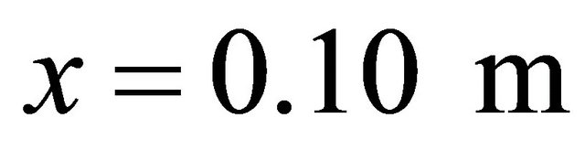 to
to 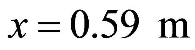 in the streamwise direction and from
  to
to 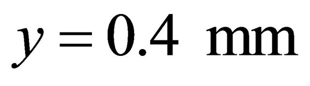 in the vertical direction. Table 2 and Figure 3" target="_self"> Figure 3 provide detailed information on the streamwise locations of boundary layer measurements. Figure 4 shows the distributions of measured surface velocity as well as the resultant acceleration parameter
  over the test model which is defined as:
 (6)
(6)
The passage-contouring device produced a gradual flow acceleration of over 0.35 m in the test model and the averaged acceleration parameter was about 7.1 × 10⁻⁵.
Table 1. Text conditions.
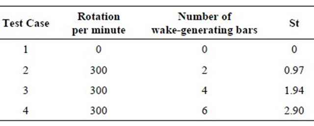
Table 2. Measurement locations.
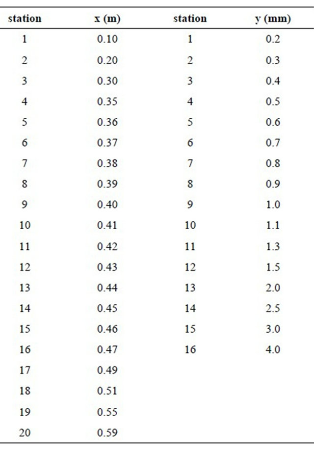
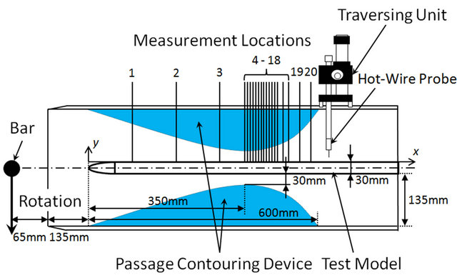
Figure 3. Passage-contouring device and measurement locations.
The peak value of the acceleration became more than 3.0 × 10⁻⁴. Figures 5 and 6 show the ensemble-averaged velocity and turbulence intensity distributions of the
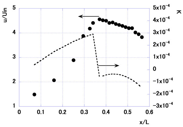
Figure 4. Measured surface velocity and acceleration parameter.
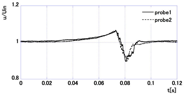
Figure 5. Velocity distribution of the bar wake.
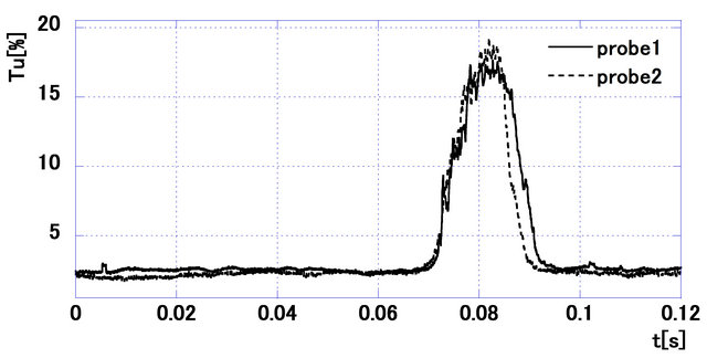
Figure 6. Turbulence intensity distribution of the bar wake.
incoming wakes respectively, measured by the hot-wire probes located  upstream of the test model. These data were normalized with the inlet velocity. The maximum wake turbulence intensity reached approximately 18%. The velocity deficit inside the wake was approximately 10% of the inlet velocity. In this study, the turbulence intensity of the transition onset at 4% was set as a criterion [12].
4. Results
4.1. Raw Signals of Velocity
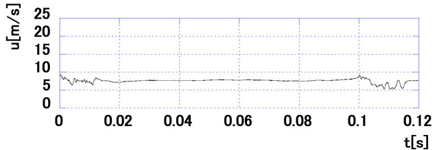
In this study, although two hot-wire probes were used, there was no definite difference in the turbulence intensity behavior between probe 1 and probe 2. Thus, only the data from probe 1 is shown. Figure 7 shows the raw signals of the velocity acquired at  for several measurement locations in the case of Test Case 2. The raw velocity signal measured at
  illustrates the wake-passing by the fluctuation. Thereafter spike-like events occurred at locations 14, indicating the initiation of the transition, followed by the abrupt completion of the transition. On the other hand, the raw signal of velocity measured at
  exhibits a fluctuating intensity regardless of time, indicating a turbulent flow.
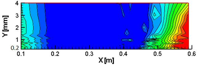
4.2. Contours of Time-Averaged Turbulence Intensity for No Wake Condition
Figure 8 shows the contours of the time-averaged turbulence intensity for the no wake condition, Test Case 1. The position of , and the turbulence intensity increased as the flow progressed downstream from there. This cause is considered, as raw signals of velocity show in Figure 7(c), the effect of an adverse pressure gradient changed the turbulent flow.
 (a)
(a)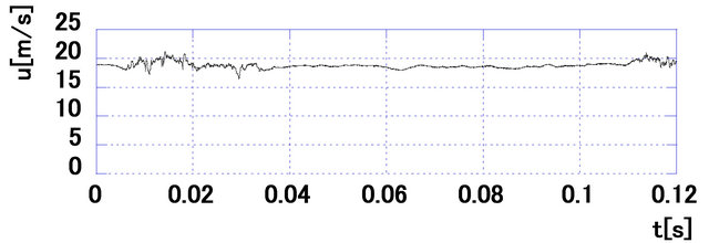 (b)
(b)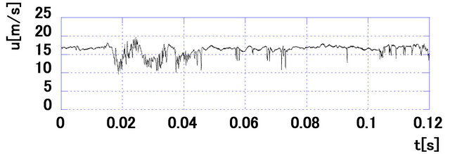 (c)
(c)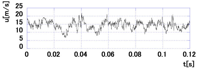 (d)
(d)
Figure 7. Raw velocity signals measured at y = 2 × 10⁻⁴ m for several locations over the test model with influence of the wake passing on the test surface (S = 0.97). (a) x = 0.10 m; (b) x = 0.30 m; (c) x = 0.45 m; (d) x = 0.59 m.

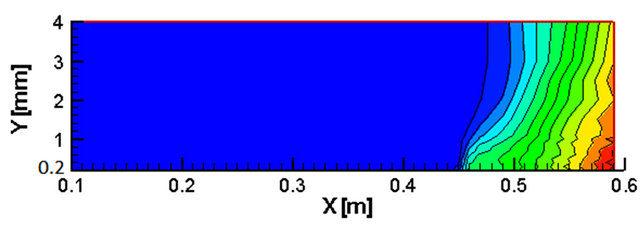
Figure 8. Contours of time-averaged turbulence intensity for no wake condition for Test Case 1.
4.3. Contours of Instantaneous Turbulence Intensity for Wake-Induced Condition
For further investigation of the wake-disturbed boundary layer, ensemble-averaged turbulence intensity contours that represent bar-wakes interacting with boundary layer are shown Figure 9. This figure represents some of the sequential snapshots during one wake-passing period T for the case with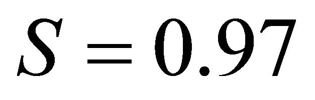 . At the instant when one barwake, which was identifiable from its high turbulence intensity, reached the most upstream measuring position at
 , there was a clear evidence showing the appearance of wake-induced turbulence zone (turbulence patch) beneath the incoming wake. As the wake was convected downward, the leading edge of the induced turbulence patch moved almost along with the wake while the trailing edge of the patch lagged behind the wake, resulting in gradual expansion of the turbulence patch in the streamwise direction. Due to the effect of the flow acceleration, however, the height of the patch remained almost unchanged. In the instant when the leading edge of the patch reached the trailing edge of the foregoing turbulence patch (
 ), another high turbulence region occurred at x/L = 0.43 - 0.47 (from location 12 to 16) designated “A”, exhibiting quick growth in the y direction (normal to the wall) due to the effect of adverse pressure gradient. A plausible explanation on this event was a high rate of turbulence spot generation at the decelerating flow regime [1].
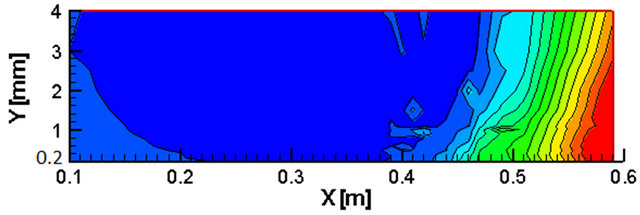
4.4. Contours of Time-Averaged Turbulence Intensity for Wake-Induced Condition
Figure 10 shows the contours of the time-averaged turbulence intensity for wake-induced flow. They were obtained by averaging the turbulence intensity in a wake-passing period. For Test Case 2 shown in Figure 10(a), the position of  at
at  was
was . For Test Case 3 show in Figure 10(b), the positions of Tu = 4% at
  and
and  in the adverse and favorable pressure gradient regions, respectively. For Test Case 4 show in Figure 10(c), the positions of
  at
at  were
were  and
and  in the adverse and favorable pressure gradient regions, respectively. For Test Cases 3 and 4, in the favorable pressure gradient region, we confirmed that the turbulence intensity increased as it went upstream.
4.5. Contours of Tu = 4% of Time-Averaged Turbulence Intensity for Wake-Induced Condition
Figures 11 and 12 show the contours of  of time-averaged turbulence intensity for a wake-induced flow on both the inner side and the outer side. In the adverse pressure gradient region, the contour of
  of the time-averaged turbulence intensity moved upstream
 (a)
(a)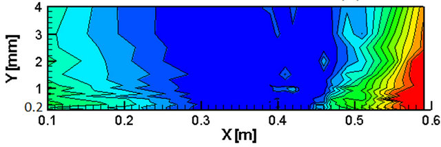 (b)
(b)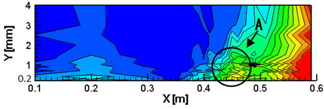 (c)
(c)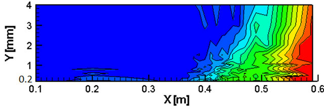 (d)
(d)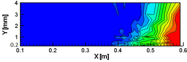 (e)
(e)
Figure 9. Contours of instantaneous turbulence intensity of the wake-disturbed boundary layer (S = 0.97). (a) t* = 0.00, (b) t* = 0.10, (c) t* = 0.20, (d) t* = 0.30, and (e) t* = 0.40.
 (a)
(a)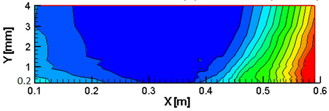 (b)
(b)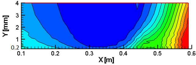 (c)
(c)
Figure 10. Contours of time-averaged turbulence intensity for wake-induced flow. (a) Test Case 2 (St = 0.97), (b) Test Case 3 (St = 1.94), (c) Test Case 4 (St = 2.90).

Figure 11. Contours of Tu = 4% of time-averaged turbulence intensity for wake-induced flow (inner side).
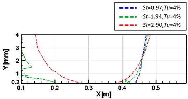
Figure 12. Contours of Tu = 4% of time-averaged turbulence intensity for wake-induced flow (outer side).
as moved upstream as the Strouhal number increased in both cases. In the favorable pressure gradient, the contour of  of the time-averaged turbulence intensity moved downstream as the Strouhal number increased in both cases.
5. Conclusions
This study experimentally investigated the wake-induced transition of flat plate boundary layers. The important findings are as follows:
1) Time-averaged turbulence intensity in the favorable gradient region increased with the Strouhal number.
2) The transition onset in the adverse pressure gradient region moved upstream as the Strouhal number increased.
3) For the wake-induced flow, in the favorable gradient region, the turbulence intensity of the wake was suppressed since the flow accelerated.
6. Acknowledgements
The authors are indebted to invaluable support from the Techno Center staff and former students Mr. S. Fujimoto and Mr. K. Takeuchi of Sophia University.
REFERENCES
- R. E. Mayle, “The Role of Laminar-Turbulent Transition in Gas Turbine Engines,” ASME Journal of Turbomachinery, Vol. 113, No. 4, 1991, pp. 509-537. doi:10.1115/1.2929110
- G. J. Walker, “The Role of Laminar-Turbulent Transition in Gas Turbine Engines: A Discussion,” ASME Journal of Turbomachinery, Vol. 115, No. 2, 1993, pp. 207-217. doi:10.1115/1.2929223
- D. E. Halstead, D. C. Walker, T. H. Okiishi, G. J. Walker, H. P. Hodson and H.-W. Shin, “Boundary Layer Development in Axial Compressors and Turbines: Part 1 of 4- Composite Picture,” ASME Journal of Turbomachinery, Vol. 119, No. 1, 1997, pp. 114-127. doi:10.1115/1.2841000
- D. E. Halstead, D. C. Walker, T. H. Okiishi, G. J. Walker, H. P. Hodson and H.-W. Shin, “Boundary Layer Development in Axial Compressors and Turbines: Part 1 of 3- LP Turbines,” ASME Journal of Turbomachinery, Vol. 119, No. 2, 1997, pp. 225-237. doi:10.1115/1.2841105
- E. Koyabu, K. Funazaki and J. Takahashi, “Boundary Layer Bypass Transition on a Flat Plate Induced by Periodic Wake Passage Affected Pressure Gradients (Effect of Free-Stream Turbulence),” Journal of the Gas Turbine Society of Japan, Vol. 29, No. 625, 2001, pp. 485-492.
- E. Koyabu, K. Funazaki and M. Kimura, “Experimental studies on Wake-Induced Bypass Transition of Flat-Plate Boundary Layers under Favorable and Adverse Pressure Gradients,” JSME International Journal Series B Fluids and Thermal Engineering, Vol. 48, No. 3, 2005, pp. 579- 588. doi:10.1299/jsmeb.48.579
- J. D. Coull, R. L. Thomas and H. Hodson, “Velocity Distributions for Low Pressure Turbines,” ASME Journal of Turbomachinery, Vol. 132, No. 4, 2010, pp. 1-12.
- K. Funazaki, N. Tanaka and M. Kikuchi, “Studies on High-Lift LP Turbine Airfoils of Aero Engines,” Transactions of JSME, Series B, Vol. 74, No. 747, 2008, pp. 2301-2310.
- X. Ottavy, S. Vilmin, M. Opoka, H. Hodson and S. Gallimore, “The Effects of Wake-Passing Unsteadiness over a Highly Loaded Compressor-Like Flat Plate,” 2002, ASME Paper GT-2002-30354.
- R. J. Volino and L. S. Hultgren, “Measurements in Separated and Transitional Boundary Layers under Low-Pressure Turbine Airfoil Conditions,” ASME Journal of Turbomachinery, Vol. 123, No. 2, 2000, pp. 189-197.
- S. J. Kline and F. A. McClintock, “Describing Uncertainties in Single-Sample Experiments,” Mechanical Engineering, Vol. 75, No. 1, 1953, pp. 3-8.
- K. Funazaki, Y. Yamashita and S. Yamawaki, “Studies on Unsteady Boundary Layers on a Flat Plate Subjected to Incident Periodic Wakes and Free-Stream Turbulence,” Journal of the Gas Turbine Society of Japan, Vol. 21, No. 81, 1993, pp. 62-69.