Open Journal of Optimization
Vol.06 No.03(2017), Article ID:79317,33 pages
10.4236/ojop.2017.63009
Mathematical Model of the Criterion of Optimization by Compensation for Designing Commercial Bottles with Lateral Surfaces of Revolution and a Straight Section along Its Silhouette
Lizandro B. R. Zegarra1*, Luis E. G. Armas2**, Aida D. Reyna3, Julio A. L. Vergara1, Fidel A. V. Obeso1
1Departamento de Matemática de la Universidad Nacional del Santa, Chimbote, Perú
2Grupo de Óptica Micro e Nanofabricação de Dispositivos (GOMNDI), Universidade Federal do Pampa, Campus Alegrete, Alegrete, Brazil
3Departamento de Matemática de la Universidad Nacional de Trujillo, Trujillo, Perú

Copyright © 2017 by authors and Scientific Research Publishing Inc.
This work is licensed under the Creative Commons Attribution International License (CC BY 4.0).
http://creativecommons.org/licenses/by/4.0/


Received: August 5, 2017; Accepted: September 23, 2017; Published: September 26, 2017
ABSTRACT
In this article, the mathematical foundations of the so called Criterion of Optimization by Compensation for designing commercial bottles with a straight section along its silhouette and with lateral surfaces of revolution is presented. Such mathematical model uses as main tools, Lagrange polynomial interpolation and Newton’s Method for Nonlinear Systems being first necessary to formulate and demonstrate a theorem. It was redesigned and manufactured a bottle of a half-liter of Fanta soda of the well-known Coca Cola Company, which uses 18.86% more material that such criterion establishes. It was expected that the redesigned bottle use 4.91% more of material with respect to what is established by the Criterion of Optimization by Compensation. However, it was reported a 13% of mistake due to important limitations that must be overcome.
Keywords:
Optimization, Modelling, Bottle Design, Environmental Pollution, Solid Residues

1. Introduction
During the production stages of a bottle until being finally sent to the consumers, the manufacturers and merchants must confront a more exigent market and society every day. The bottle has to satisfy not only the necessity of containing, protecting, preserving, commercializing and distributing merchandise, if not also, of retraining, decrease of the ecological impacts and minimization of costs. Therefore, it is necessary to design appropriate bottles according to necessities above indicated, making this evident the necessity of generating and transmitting the knowledge of science and technology, in which the concept of optimization is of great importance. For instance, Fletcher [1] and Pierre [2] describe optimization methods that are currently most valuable in solving real-life problems.
Up to now, there has not been found studies about a clear mathematical model of an optimization method of a bottle with a lateral surface of revolution and a straight section along its silhouette. In the case of PET bottles, there are some studies about optimizing and redesigning the whole or part of the body of them by using different software programs. Masood and KeshavaMurthy [3] have reported the process, design and optimization of a bottle shape using Pro/Engineer Parametric Modelling Software and Pro/Mechanica Finite Element Software (FES); Demeril and Dave [1] have used numerical modelling with finite element analysis (FEA) techniques to redesign the petaloid base of bottles to improve stress-crack resistance. An experimental design based on an algorithmic partial cubic method was employed. Quinchung et al. [4] have optimized the structure of the PET bottle in order to increase the buckling load, based on the Abaqus/ Explicit computer program. Moreover, according to the stress contour of PET bottle obtained by Abaqus, plastic distribution of PET bottle was optimized in order to improve the efficiency of PET material and reduce the weight of the PET bottle. In addition, Mohammad [5] described the formulation of the mathematical model of the PET thermoplastic material for FEA drop-test simulation. Finally, Silva et al. [6] have designed and optimized a PET bottle through parametric computer aided design software (solidworks) and finite element method analysis, allowing the simulation of the blowing process from data input to the process variables listed in the available literature.
On the other hand, for aluminum bottles, Han et al. [7] have used numerical simulation and mathematical programming to optimized a cylindrical shell body of an aluminum can (volume: 500 ml), which was triangulated as one of the expectant choices of crushable cans for being folded down easily and safely for recycling. At the same way, Han et al. [8] have applied the structural optimization technique, to aluminum beverage bottle design, based on nonlinear finite element analyses to know the influence of the design parameters on the buckling strength and the stiffness of the bottom under an axial load and internal pressure, respectively. Similarly, Han et al. [9] have also performed multi-objective optimization of a two-piece aluminum beverage bottle considering tactile sensation of heat and embossing formability. Karl et al. [10] have performed simulation of the filling of PET bottles with a volumetric swirl chamber valve on the basis of calculations models and experiments. Hopmann et al. [11] have provide a sism tiao mulative approach to determine a well-adapted preform and bottle design as well as corresponding process parameters. For this, a three-dimensional simulation of the stretch-blow molding process was used within an iterative optimization routine. At the same way, numerical modelling and optimization of the production process of glass bottles have been the topic of several papers [12] [13] [14] [15] [16] [17] .
Therefore, since most containers whose shapes are determined by surface of revolution and manufactured from plastic or metal material, the enterprises that decide to apply criterion of optimization on its manufacture, could try to reach the following achievements: reduction of rubbish, saving energy, decrease of the negative environmental impact and hence a friendly environmental image.
In this work, we report a mathematical model of the Criterion of Optimization by Compensation proposed by Reyna and Moore [18] in order to design commercial bottles with lateral surfaces of revolution and a straight section along its silhouette. With the aim of designing and manufacturing bottles using the less amount of material in their fabrication, it can avoid so environmental pollution by solid residues. Since the expenditure of material is proportional to the area of a bottle, to design a bottle by using the lesser as amount of material as possible, means that the superficial area of the bottle have to be minimized. For example, to design a cylinder of minimal area is very easy since it is possible to find its area as a function of its radius and then in using differential calculus to get the radius and height of the cylinder that makes the area of the cylinder a minimum. In the case of any container (bottle in particular) with lateral surface of revolution and a predetermined silhouette, to get a mathematical relation similar to the case of the cylinder, in general is not possible. In this case, that the Criterion of Optimization by Compensation becomes appropriate.
Such Criterion of Optimization by Compensation tells us that in order to design a bottle with a minimal total superficial area, it must first design a cylinder with a minimal total superficial area. From the cylinder, it must be get the shape of the bottle by removing certain solid parts of the cylinder. With the solid parts removed, it must be formed a cylinder whose volume is equal to the sum of the volumes of the solid parts removed from the initial cylinder. The lateral surface area of the formed cylinder must be equal to or less than the sum of the outer surface areas of the solid parts removed from the initial cylinder. This new formed cylinder has to fit the straight section of the bottle that is being designing. Since de cylinder has a minimal area, it is optimized, and at a beginning, the superficial area of the bottle is optimized too. Indeed, theorem 2.1 (see below) shows that the area of the bottle results to be less than that of the cylinder. However, this is only a descriptive fact and a mathematical modelling turns out to be necessary. Then, this work presents a mathematical modelling as the one required, according to the Criterion of Optimization by Compensation.
2. Theory
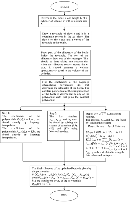
Flow diagram of the Optimization method for designing an optimized bottle of volume V. The starting point is a cylinder of minimal area of volume V. Following the Criterion of Optimization by Compensation according to steps 1, 2,…, , where k is a finite number, the final silhouette of the optimized bottle can be found. From this, the three dimensional bottle is obtained.
2.1. Criterion of Optimization of Containers with a Straight Cylindrical Shape
To design a container with a straight cylindrical shape and of a certain volumetrically capacity in using a smaller amount of material, lead us to determine a minimum of the following function
(1)
where V, A and r are the volume, total area and radius of the cylinder respectively.
Deriving the function with respect to r and equaling to zero we have that
Solving this equation with respect to r
(2)
Which is a critical point for the function given in Equation (1)
But
(3)
By replacing (2) in (3)
Which is major than zero. This means that the value of r given by Equation (2) corresponds to a minimum and which let us determine the height h of the cylinder in using , equal to
(4)
As it can be seen in this case, it is not difficult to get the values of r given by Equation (2) and h given by Equation (4) which let us minimize the area of a cylinder for a given value of its volume V. Furthermore Equation (3) tell us that
Equation (1) is always concave above because , . This
means that
2.2. Criterion of Optimization by Compensation
In the case of designing containers with a non-cylindrical shape as it can be the general case, of a bottle, its silhouette could result whimsical due to aesthetic considerations as many others, so it is impossible to write an Equation (function), as in the case of the cylinder discussed in Section 2.1. Therefore, in order to solve this apparent difficult, we will use the Criterion of Optimization by Compensation proposed by Reyna and Moore [18] . This optimization criterion consists in designing first a cylinder with a minimal area for a given volume in using Equations (2) and (4) and then redistributes the total volume and area that will be removed from de cylinder in order to get the desired shape of the bottle that we wish to manufacture. At the end of the process, the volume of the resultant bottle must be equal to that of the original cylinder, where the area of the resultant bottle could be less than that of the cylinder, as it is shown in theorem 2.1 below. Now, the unique proposition given in [19] tell us that the area of a cylinder of minimal area is among the area of a sphere and the area of a cube having all of them the same volume. But, the area of the bottle turns out to be less than that of the cylinder of minimal area, so we have the area of a bottle closer to the area of a sphere than the area of a cylinder of minimal area. Of course, the volumes of the bottle, cylinder of minimal area and sphere are the same. Since the sphere is considered as a geometric object with maximum volume and lesser area, the Criterion of Optimization by Compensation turns out to be a good method for optimizing.
An outline of the Criterion of Optimization by Compensation, in order to minimize the area of a bottle, keeping a constant volume is as follow:
1) Know the volumetric capacity V of the bottle that will be optimized;
2) Optimize the total area of a cylinder whose volumetric capacity is V;
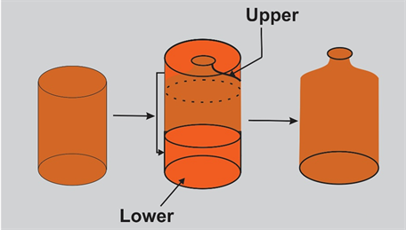
3) In each zone of the optimized cylinder where will be modified (Figure 1(a)) in order to get the desired shape of the bottle, it must be removed a solid which is enclosed by an external surface, the surface of the cylinder, and internal surface, the surface of revolution that will give the shape to the bottle. See in the upper part of Figure 1(b) signed with the arrow. Calculate the difference of areas between the cylindrical surface and the surface of revolution that both enclose the solid that was removed. With this difference must be formed a cylinder without bases whose volume must be equal approximately to the volume that was removed (see Figure 1(b));
 (a) (b) (c)
Figure 1. (a) Optimized cylinder with a volume V from which an optimized bottle will be obtained; (b) Cylinder with an upper region that will be lost and recovered in the lower region; (c) Bottle after the application of the optimization criterion. Adapted with permission from Reyna and Moore [18] . Copyright 2016 ECI.
4) Fit the cylinder without bases, obtained in the step 3, in the cylindrical zone of the optimized cylinder. In this way, it is possible to obtain an optimized bottle with lateral surface of revolution (see Figure 1(c)).
The theorem below is based on the Criterion of Optimization by Compensation. This theorem tell us that it is possible to deform a cylinder of volume and minimal area to a solid of revolution of volume and area such that and . This theorem is formulated in order to show in particular that the area of a bottle could be less than the corresponding minimal area of a cylinder, both enclosing the same volume, so that the optimization of the bottle is better.
Theorem 2.1 There exists a solid of revolution of the non-convex type whose surface is less than the surface of a right circular cylinder of minimal area, keeping both of them the same volume.
Proof
Figure 2 shows the scheme to be used in order to prove the theorem given above.
From scheme of Figure 2 we have:
(5)
Due to the Criterion of Optimization by Compensation,
(6)
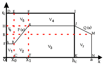
Figure 2. Schema according to the criterion of optimization by compensation. and correspond to the height and radius of a cylinder of volume and minimal area which is generated when the rectangle ODIK rotates around the x-axis. From Equations (2) and (4), we have that . and are polynomials of first degree whose coefficients must be found. are the volumes generated when the regions given by the correspondent closed polygons OABC, CBGT, TGJK, GFIJ, BEFG, ADEB and KJMN, rotate around the x-axis. , are the areas generated when the correspondent segments OA, AB, BG, GJ, JM and MN, rotate around the x-axis. The value of must be found. and are values that must be freely given in such a way as to allow us to determine an acceptable value for .
replacing Equation (6) in (5)
(7)
We have as well that,
(8)
(9)
(10)
(11)
(12)
(13)
(14)
By replacing Equation (13) in (10)
(15)
Then,
(16)
By replacing Equation (14) in (12),
(17)
Then,
(18)
By replacing Equations. (8), (9), (11), (16) and (18) in (7),
(19)
Let be such that,
(20)
Where,
(21)
(22)
(23)
(24)
(25)
(26)
(27)
Deriving Equation (13),
(28)
Deriving Equation (14),
(29)
Replacing Equations (13) and (28) in (23) and integrating,
(30)
Then,
(31)
Replacing Equations (14) and (29) in (25) and integrating,
(32)
Then,
(33)
Replacing Equations (21), (22), (24), (26), (31) and (33) in (20),
(34)
Now, the conditions that the polynomials and must satisfy are:
(35)
(36)
(37)
(38)
From Equations (35) and (13),
(39)
From Equations (36) and (13),
(40)
From Equations (37) and (14),
(41)
From Equations (38) and (14),
(42)
Taking into account Equations (19), (34), (39), (40), (41) and (42) we get the following system of equations,
(43)
(44)
(45)
(46)
(47)
(48)
Hence, we have six equations in five unknowns.
From Equations (43) and (44),
(49)
(50)
From Equations. (45) and (46),
(51)
(52)
By replacing Equations (15) and (17) in (47),
(53)
By replacing Equations (49), (50), (51) and (52) in (53) and simplifying,
(54)
Equation (54) is an equation in the unknown parameter a.
By replacing Equations (30) and (32) in (48)
(55)
By replacing Equations (49), (50), (51) and (52) in (55),
(56)
Equation (56) as well as Equation (54), is an equation in the unknown parameter a.
Since we have a theorem of existence, we solve numerically Equation (54) in the unknown parameter a in using the testing data , , , , , and . Here, from Equa-
tions (2) and (4) and the value is arbitrary. The rest of
values for and are given heuristically by looking Figure 2 and according to the Criterion of Optimization by Compensation. This let us find . With this data, the area and volume of the solid of revolution that is generated when the region enclosed by the polygonal OABGJMN and x-axis of Figure 2, rotates around x-axis, are equal to and respectively.
The minimal area of the cylinder of revolution that is generated when the region enclosed by the rectangle ODIK rotates around the x-axis, is equal to , while its volume is equal to which is the same value for the solid of revolution. So, we have and which prove the theorem.
Equation (56) led us to a no wished solution since increase the volume of the solid of revolution to such that the surface of minimal area of the cylinder is . Say, we have and .
2.3. Mathematical Model of the Criterion of Optimization by Compensation for Designing Commercial Bottles with a Straight Section along Its Silhouette
In this section, the mathematical model of the criterion of optimization by compensation for designing commercial bottles with lateral surfaces of revolution and a straight section along its silhouette is presented. The start point is the schema shown in Figure 3, which is based in the criterion of optimization by compensation seen in the xy-plane.
The mathematical model taking into account the Criterion of Optimization by Compensation is as follows: consider the schema (shown in Figure 3) corresponding to a general bottle with a straight section along its silhouette, where , are volumes generated when the regions below the curves represented by the non-constant polynomials of certain

Figure 3. Schema to get a mathematical model in using the Criterion of Optimization by Compensation. When the rectangle with vertices and rotates around the x-axis, the cylinder of minimal area is to be obtained. When the curve described by the polynomials that must be determined in using interpolation when a set of points is given, rotates around the x-axis, the bottle must be obtained. Here, and are known constants. are the polynomials that describe the silhouette of the bottle. and are described on the text.
degree rotates around the x-axis. The value of depends on the number of polynomials needed to complete the shape of the silhouette of the bottle out of the rectangle with vertices , , and . are volumes generated when the regions above of the polynomials , rotates around the x-axis. and are volumes below and above the constant polynomial . Then, from Figure 3
(57)
where is the volume of the cylinder of minimal area with radius and height which is generated when the rectangle with vertices and rotates around the x-axis (see Figure 3). By Criterion of Optimization by Compensation
(58)
Putting Equation (58) in (57)
(59)
But,
(60)
(61)
(62)
(63)
(64)
(65)
(66)
Putting Equations (60)?(66) in (59), we have finally,
(67)
Equation (67) is a fundamental equation derived from the Criterion of Optimization by Compensation.
Now let , , , , , , , be,
the polynomials that are shown in Figure 3, where the coefficients of these polynomials are unknowns. Thus, the Optimization problem can be formulated as follows: given the equation
(68)
Subject to the following conditions:
(69)
(70)
(71)
(72)
(73)
(74)
(75)
(76)
(77)
(78)
(79)
(80)
(81)
(82)
(83)
(84)
where in Equations (70)-(78) are constant ordinates given by the designer. On the other hand, in order to give the shape of the silhouette of the bottle, , , ; , , ; , , , are also given by the designer such that each of them determines a set of points through which the polynomials obtained by interpolation, passes respectively. Similarly, the , , ; , , ; , , , ; are also given by the designer, such that each of them determines a set of points through which the polynomials obtained by interpolation, passes respectively. These polynomials are such that their corresponding polynomials by translation according to, fit with the remaining part of the bottle in the interval . The and are constants given by the designer, while and are the radius and height of a cylinder of minimal area. We must find ; ; ; ; ; ; ; ; ; such that the area of the bottle of volume is less or equal than the area of a cylinder of minimal area according to the theorem given above.
Solving the Problem of Optimization
We can solve the optimization problem in using Lagrange polynomial interpolation and Newton’s Method for Nonlinear Systems according to the following steps:
Step 1 Find the constants ; ; ; ; ; ; ; , in using Lagrange interpolation, say, by determining the coefficients of the Lagrange interpolating polynomial in each case respectively. These coefficients are the constants we are trying to find.
Step 2 The and can be found by solving the system of Equations (85), (86) and (87) given below, in using the Newton’s Method.
(85)
where,
are integrals that correspond to the polynomials
, and can be calculated as well as .
(86)
(87)
Step 3 and1 can be found by solving the system of equations:
can be calculated in using the data calculated in step 2.
Step 4 and can be found by solving the system of equations:
can be calculated in using the data calculated in step 3.
Step k and can be found by solving the system of equations:
can be calculated in using the data calculated in step .
Step k+1 and can be found by solving the system of equations:
can be calculated in using the data calculated in step k.
The number of unknown coefficients of the polynomials depends on the number of points that were arbitrary chosen, in order to get a Lagrange polynomial that must describe the silhouette of the bottle. Hence, we must be careful when the number of points are chosen, since the polynomial in that region could present slight oscillations and not describing the shape of the silhouette of the bottle in that region, as shown in Figure 4. If this were the case, we must try to choose other points by varying slightly some points of the initial set of points until the oscillations have vanished. Polynomial oscillation could be present when a number of chosen points are not appropriated in order to get a Lagrange polynomial interpolation. Therefore, in order to get a desirable solution for the problem of optimization and choose a set of points in such a way that the poly
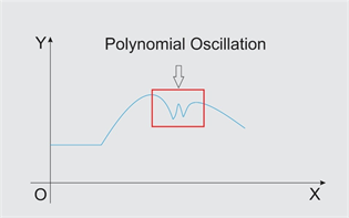
Figure 4. Schema showing the polynomial oscillations when the chosen points are not appropriated to get the Lagrange interpolation. This happens when the number of points chosen is great.
nomials should be free of oscillations, we must use a computer program (optimizer of five sections).
2.4. Application of the Criterion of Optimization by Compensation
As an application of the criterion by compensation, a bottle of Fanta soda of the Coca Cola Company was considered, as shown in Figure 5. The characteristics of the bottle are: Type of the product that it contains: carbonated drink; Factory: Coca Cola company; volume of the bottle: 537.5 ml; weight of the empty bottle without its cap: 25.18 g; material from which the bottle is manufactured: Polyethylene terephthalate (PET); base of the bottle: petaloid base of five cavities.
We first analyse the real bottle, in order to determine its superficial area mainly. In fact, after cutting along the bottle through the middle and putting half of it in a coordinate system, previously drawn on a millimetered paper, the x and y coordinates of the silhouette of the real bottle are shown in Table 1:
Figure 6(a) shows for the real bottle, the interface of the computer program elaborated in the high-level programming language MATLAB. This computer program has five options: interpolate, volume, area, surface of revolution and optimize in order to perform the tasks. The calculations are performed by considering the bottle with a flat base. Adjustments are made in Input Data of each section. In this case, it was considered five sections for the bottle. In Optimizer, the volume of the bottle to be optimized must be entered. As a result, in using Equations (2)-(4), we get optimum results for the cylinder, such as: radio, height and area. In Output Data of Figure 6(a) are shown the results of the volume and area of the bottle, according to the adjustments that were made in Input data of each section. When the optimization is being performed the value of the area varies until get approximately the value of the area obtained in Optimum results for the cylinder, keeping approximately constant the value of the volume in Optimizer (see Figure 6(a)). In using the computer program and with the data of the Table 1, the real bottle in three dimensions is shown in Figure 6(b). As, it can be seen from the results of the calculations in using the
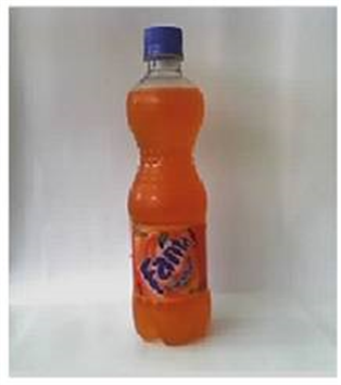
Figure 5. Bottle of Fanta soda, from the Coca-Cola Company, used to apply the application of the Criterion of Optimization by Compensation.

Figure 6. Real bottle, (a) Silhouette of the real bottle according to the data of the Table 1. It is shown the sections S1, S2…S5, according to data in Input Data of Each Section in Optimizer of Five Sections. In Optimizer, the volume V of the bottle is entered in order to obtain the optimum radius, optimum height and optimum area of the cylinder which are visualized in Optimum Results for the Bottle. In Output Data, for the bottle, the volume and area of the bottle are visualized when the curves in corresponding sections S1, S2…S5 rotates around the x- axis and which generate the bottle; (b) view of the real bottle in three dimensions.

Table 1. Coordinates of the silhouette of the real bottle seen in a Cartesian coordinate system of the xy plane. Section 1 (S1), corresponds to the lip of the bottle, Section 2 (S2), section 3 (S3), section 4 (S4) and section 5 (S5) correspond to the form of the bottle.
computer program, the optimum area of the bottle according to the Criterion of Optimization by Compensation must be 365.96 cm2 when the base of the bottle is flat.
It is worth to emphasize that, the volume of 551.63 cm3 in Output Data, of Figure 6(a), for the bottle exceeds 537.5 cm3 because the program calculates the volume of the bottle with flat base. By measuring the volume of the cavities of the petaloid base (base of the real bottle) in laboratory by using water for filling such cavities, it is found a total volume of 14 cm3 approximately that have to be subtracted from 551.63 cm3. So we have 537.63 cm3 which is a good approximation of the volume of the real bottle. Similarly, the area 435.972 cm2 in Output Data for the bottle is due to fact that the program calculates the area of the bottle by considering it with flat base. By calculations made apart in the zone of the petaloid base in order to determine its area by approximation by triangles and circles as shown in Figure 7, we find that the area of the bottle with petaloid base is 435.23 cm2, so that the difference in areas between the bottle with flat base and petaloid base is not significant.
In order to redesign the bottle, it is necessary to give some points through which the silhouette of the redesigned bottle passes. These points are given by the designer and are shown in Table 2, being shown a set of them in Figure 8 by circles in sections S1, S2, S3, S4 and S5. The task is to determine by Lagrange interpolation the polynomials that pass through these points. The number in the x-axis, is the right extreme of the section S4 which is a straight line, and left extreme of section S5 represented by the polynomial . This number must be determined by moving section S5 to the right or left according to the sign of , positive or negative in as it is shown in Figure 8. These polynomials are the starting points to get the final polynomials that determine the silhouette of the redesigned bottle and hence optimized. As it can be seen

Figure 7. Approximation by triangles and circles in order to determine the area of the petaloid base of the bottle.

Figure 8. Silhouette of the redesigned bottlein using a set of pointsof Section 1 (S1), Section 2 (S2)… Section 5 (S5) shown in Table 2.
Table 2. Coordinates of the silhouette of the redesigned bottle seen in a Cartesian coordinate system of the xy plane. Section 1 (S1) corresponds to the lip of the bottle; Section 2 (S2), Section 3 (S3), and Section 5 (S5) correspond to the form of the bottle.
according to the development of the model in Section 2.3, in general the polynomials are susceptible of changing, depending if some of are zero or different of zero. In this particular case we have only from and we will find that , so that the Lagrange polynomials of the redesigned bottle will be equal to the Lagrange polynomials of the optimized redesigned bottle.
It is worth to emphasize that, the coefficients of the polynomials, in Table 3, are expressed in the form of decimals in order to decrease distortions in the design of the bottle, optimization and during passing data to the CNC lathe. Greater the number of considered decimal places better will be the design. These criteria are taken into account in all the calculations that are made in all the process of optimization and must be presented in this way.
In order to get the optimized redesigned bottle, rest to find the polynomial from that fit correctly with the design of the silhouette of the bottle. To do this we put in Table 2, instead of 9.71 and instead of 12.01 and a new Table with new values for and must be found.
Equations (73) and (74) with , where , and in using the polynomial become,
, from Equation (74),
(88)
, from Equation (73),
(89)
By looking Figure 8 we see that , , and , , . In using the data of Table 3, Equation (67) can be written as,
where .
By numerical integration of the first two integrals and taking into account that , we have,
Table 3. Polynomials according to the points given in Table 2 corresponding to Section 1 (S1), 2 (S2), 3 (S3), 4 (S4) and 5 (S5) of the redesigned bottle.
From which
(90)
Since
where integration was performed analytically, Equation (90) becomes finally,
(91)
Now, must be solved the system of Equations (88), (89) and (91).
Since a system of three nonlinear equations in three unknowns has been obtained, must be solved numerically in using the Newton’s Method for Nonlinear Systems, whose interface Solver For System of Nonlinear Equations (SNLEs) shows us the results of the values for the unknowns after perform 5 iterations (see Figure 9). To solve the system, Equations (88), (89) and (91) are renamed as and , where:
Additionally, we need the elements of the Jacobian matrix, which are:

Figure 9. Solver for System of Nonlinear Equations based on Newton?Raphson numerical method to find the unknowns parameters of Equations. (88), (89) and (91). These Equations were renamed as , and (see Enter F). This figure also show the Enter Jacobian Matrix ( , , , , , , , and ); Enter initial points ( , and ) as well as the Approximations to roots.
In order to enter Equations (88), (89), (91) and the elements of the Jacobian matrix to the SNLEs, in Matlab language, we change to an equivalent form. Then, taking into account and , we have
Figure 9 shows the SNLEs, where it is possible to see the entry functions , and ; Jacobian matrix , , , , , , , and ; initial points , and as well as the approximations to roots.
In Approximations to roots of the Solver for System of Nonlinear Equations, we can see that , and . The values of , , , and , in Figure 9, are similar to values of Table 2; and , , , similar to values of Table 3. With these results, and in using the Optimizer of Five Sections, we get the polynomials for the optimized redesigned bottle shown in Lagrange polynomial coefficients of Figure 10, and which are shown in Table 4.
Therefore, with the data of Table 2 where and and following the same procedure that was made for the real bottle, the results for the redesigned bottle, after applying criterion of optimization by compensation, are shown in Figure 10.
In Output data of this figure, we can see that we can manufacture a bottle with an area of 363.588 cm2 less than 365.96 cm2 specified in optimum area of optimum results for the bottle, which is in accordance with theorem 2.1 and similar results reported by Reyna and Morales [19] .
When considering a petaloid base for the bottle of Figure 10, and according to the design of a new petaloid base following similar calculations to that made

Figure 10. Optimized redesigned bottle with flat base, (a) Silhouette of the optimized redesigned bottle according to the data of Table 2. It is shown the sections S1, S2… S5, according to data in Input Data of Each Section in Optimizer of five Sections. In Optimizer, the volume V of the bottle is entered in order to obtain the optimum radius, optimum height and optimum area of the cylinder which are visualized in Optimum Results for the Bottle. In Output Data for the bottle the volume and area of the bottle are visualized when the curves in corresponding sections S1, S2…S5 rotates around the x-axis and which generate the bottle. The coefficients of the polynomials that represent each curve of each section S1, S2…S5 are placed on the Lagrange Polynomial Coefficients (shown in Table 4). Theseresults were obtained following the Flow diagram of the Optimization method for designing an optimized bottle of volume V; (b) view of the optimized redesigned bottle in three dimensions.
Table 4. Section 1 (S1), 2 (S2), 3 (S3), 4 (S4), and 5 (S5) of the optimized redesigned bottle with its corresponding Lagrange Polynomials that draw the silhouette of the bottle according to Table 2, where and .
for the real bottle (see Figure 6), the area of the bottle is modified from 365.96 cm2 to 366.17 m2.
Table 4 shows the Lagrange polynomials, of each section, of the optimized redesigned bottle. We can see similar results to that given in Table 3, which means that the optimization criterion by compensation works very well.
3. Results and Discussions
On the basis of the Criterion of Optimization by Compensation it was obtained a mathematical model that let us optimize (minimize) the superficial area of a bottle with a straight section along its silhouette. The minimal area that this mathematical model let us obtain is in the sense that it tends to the area of the sphere which is considered as geometric object with maximal volume and less area. Say, in general the area of the bottle is between the area of the sphere and the area of the cylinder. This is not difficult to show in using proposition presented in [11] that establishes the inequality enclosing these areas the same volume. If we build a bottle from a cylinder of minimal area according to the Criterion of Optimization by Compensation we obtain the inequality . In this sense, we are optimizing. We really don’t know the absolute minimum for the area of the bottle being this an open problem.
Results of the application of the Criterion of Optimization by Compensation for the case of the half-liter bottle of the Fanta soda, are summarized in Table 5. It can be seen that the real bottle is made in using 25.18 g of PET plastic to enclose a volume of 537.5 cm3 with a superficial area of 435.23 cm2 approximately. However, in using the Criterion of Optimization by Compensation for almost the same volume (537.63 cm3), the area can be reduced to 366.17 cm2 (with petaloid base) so that it is necessary only 21.185 g of PET plastic keeping the original thickness of the wall of the bottle. It is worth to emphasize that 21.185 g was obtained using a rule of three with the data of Table 5 keeping constant the thickness of the bottle, which is not considered as a parameter of design. It was optimized the given geometric shape of the bottle. Consequently, the real bottle of Fanta soda has a mistake of 18.86 % (This value was obtained by using the re-
lation ) respecting to what
is established by the Criterion of Optimization by Compensation and, it has 69.06 cm2 more superficial area or it uses 3.995 g more of PET plastic. In indications such as * and ** are specified that the results 366.17 cm2 and 537.63 cm3 are
Table 5. Comparison between the results of the real and the optimized bottle.
due to the petaloid base of the bottle. The difference in areas between the bottlewith flat base and petaloid base is not significant in the present work.
The cost that it is paid when the optimization is achieved in using the Criterion of Optimization by Compensation is that the height of the bottle diminishes and a widening happens. The view at scale of the real bottle and the redesigned bottle optimized in extreme is shown in Figure 11. It can be seen that the height of the redesigned bottle is almost half of the real bottle, but fatter in order to compensate the loss of volume, keeping so the same volume of the real bottle.
Since no necessarily, an optimization in extreme must be achieved, it was attempted to manufacture a bottle with a mistake of 4.91% considered arbitrarily by the designer, say, with an area of 383.916 cm2 (This value is obtained by using
the relation , where
the area of the optimized bottle is 365.96 cm2). Such attempt of manufacturing the bottle was achieved with certain limitations such as:
1) It was impossible to find preforms of PET plastic of 23.25 g approximately, as it was required by calculations.
2) It was impossible to find preforms of PET plastic whose design must be according to the
length of the lip of the bottle as it is required in the design.
3) The mechanism of exportation of data, to the numerical control lathe distorted the data. So, volume and area of the bottle were slightly altered.
Table 6 shows coordinates of the silhouette of the manufactured bottle in a Cartesian coordinate system of the
In Figure 12 we can see in Output data that the area of the bottle to be manufactured is 383.916 cm2, while the area of the bottle in Optimum results is

Figure 11. View at scale of the real and redesigned bottle. Adapted with permission from Reyna and Moore [18] . Copyright 2016 ECI.

Figure 12. Manufactured bottle, (a) Silhouette of the manufactured bottle according to the data of Table 6. It is shown the sections S1, S2…S7, according to data in Input Data of Each Section in Optimizer of Seven Sections. In Optimizer, the volume V of the bottle is entered in order to obtain the optimum radius, optimum height and optimum area of the cylinder which are visualized in Optimum Results for the Bottle. In Output Data, for the bottle, the volume and area of the bottle are visualized when the curves in corresponding sections S1, S2…S7 rotates around the x-axis and which generate the bottle. The coefficients of the polynomials that represent each curve of each section S1, S2…S5 are placed on the Lagrange Polynomial Coefficients (shown in Table 7). These results were obtained following the Flow diagram of the Optimization method for designing an optimized bottle of volume V; (b) view of the manufactured bottle in three dimensions.
Table 6. Coordinates of the silhouette of the manufactured bottle seen in a Cartesian coordinate system of the xy plane. Section 1 (S1) corresponds to the lip of the bottle, Setion 2 (S2), Section 3 (S3)…Section 7 (S7) correspond to the form of the bottle.
365.960 cm2 being in both cases when the base of the bottle is flat. This means that there is a mistake of 4.91% with respect to optimum results. As a consequence of inserting to the bottle a petaloid base plus the limitations stated above the mistake increase as it is indicated below.
Table 7 shows the Lagrange polynomials, of each section, of the manufactured bottle which were obtained following the same procedure to obtain Table 4.
The above last limitation (number 3) allowed us to obtain a bottle whose geometric design had a mistake of 13% (This value was obtained by direct measurement of the area of the mold of the bottle and by using the formula
, where the area
of the optimized bottle is 365.96 cm2 according to Optimum results for the bottle of Figure 12). The limitation, numbered as 1, caused that the thickness of the wall of the bottle resulted be 75% of that of the real bottle because a preform of 22 g of PET plastic was used. In spite of the limitations, a good bottle was obtained as shown in Figure 13. In this Figure we can see: a) the corresponding mold that was fabricated to manufacture the redesigned Fanta soda bottle of the Coca Cola company, b) comparison between the real (higher) and redesigned (smaller) bottle. Our results are in accordance with the literature, for instance, Silva et al. [6] have reported a reduction of 21% of PET material (weight of 4.6 g) of a bottle of 22 g, using simulations based on finite element method (FEM). On the other hand, Hung et al. [20] have reported a reduction of the weight of a bottle, with a volume of 500 ml, from 27 g to 22.3 g using numerical simulations, where thickness and pattern of the bottle were changed in order to reduce the weight of the bottle. At the same way, Hopmann et al. [11] have also reported a reduction of the weight of a 0.5 liter PET bottle of Krones AG, Neutraubling, Germany, from 18.5 g to 15.5 g. For this aim, they have developed a simulative approach to determine a well-adapted preform and bottle design with its corresponding process parameters. Therefore, a three-dimensional simulation of the stretch-blow molding process was used within an iterative optimization routine. Their bottles were manufactured on a stretch-blow molding machine LB1 (Krones AG, Neutraubling, Germany), with a changed wall thickness.
Therefore, according to this reports, we can note that, in all cases the wall
Table 7. Lagrange polynomials of the manufactured bottle obtained via interpolation according to data of Table 6 and in using Optimizer of seven sections.
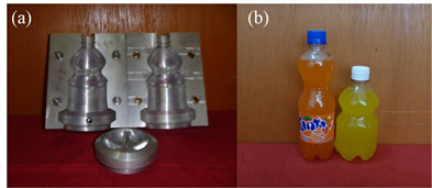
Figure 13. (a) Mold used to manufacture the redesigned bottle of Fanta soda, and (b) comparison between the real (higher) and redesigned (smaller) bottle.
thickness of the bottles was changed, and the weight of the bottle reduced in average~4.0 g, similarly to the found results in this work. However, in this work the wall thickness of the bottle have to remain unchanged.
4. Conclusion
In summary, we propose the mathematical foundations of the so-called Criterion of Optimization by Compensation and in using this, an optimized and redesigned half-liter bottle of Fanta soda of the well-known Coca Cola Company, was manufactured. This manufactured bottle was designed with a mistake of 4.91% with respect to what such criterion of optimization stablishes. However, it was reported a mistake of 13% in each manufactured bottle due to important technical limitations listed above that must be overcome. In general, in spite of such limitations a good bottle was obtained with such 13% of mistake, resulting the thickness of the wall of the bottle 75% of that of the real bottle because a preform of 22 g of PET plastic was used, instead of a preform of 23.25 g as it was required.
Acknowledgements
The authors would like to thank Universidad Nacional del Santa of Peru for its financial support in the development of the present research and the Brazilian Agency CNPq for its partial financial support. Process No 460733/2014?1.
Cite this paper
Zegarra, L.B.R., Armas, L.E.G. Reyna, A.D., Vergara, J.A.L. and Obeso, F.A.V. (2017) Mathematical Model of the Criterion of Optimization by Compensation for Designing Commercial Bottles with Lateral Surfaces of Revolution and a Straight Section along Its Silhouette. Open Journal of Optimization, 6, 115-147. https://doi.org/10.4236/ojop.2017.63009
References
- 1. Demeril, B. and Dave, F. (2009) Optimization of Poly (Ethylene Terephthalate) Bottles via Numerical Modeling: A Statistical Design of Experiment Approach. Journal of Applied Polymer Science, 114, 1126-1132. https://doi.org/10.1002/app.30644
- 2. Pierre, D.A. (1987) Optimization Theory with Applications. Dover Publications, New York.
- 3. Masood, S.H. and Keshava Murthy, V. (2005) Development of Collapsible PET Water Fountain Bottles. Journal of Materials Processing Technology, 162-163, 83-89. https://doi.org/10.1016/j.jmatprotec.2005.02.176
- 4. Qingchung, H., Wenjian, S., Yanhui, L. and Yongsheng, W. (2012) Structural Optimization and Light-weight of PET Bottle Based on Abaqus. Advanced Materials Research, 346, 558-563.
- 5. Mohammad, K.H. and Abunawas, A. (2010) Suitable Mathematical Model of PET for FEA Drop-Test Analysis. International Journal of Computer Science and Network Security, 10, No. 5.
- 6. Silva de Miranda, C.A., Drummond Camera, J.J., Monken, O.P. and Gouvea, S. (2011) Design Optimization and Weight Reduction of 500 mL CSD PET Bottle through FEM Simulations. Journal of Materials Science and Engineering B., 1, 947-959.
- 7. Han, J., Yamazaki, K. and Nishiyama, S. (2004) Optimization of the Crushing Characteristicsof Triangulated Aluminum Beverage Cans. Structural and Multidisciplinary Optimization, 28, 47-54. https://doi.org/10.1007/s00158-004-0418-8
- 8. Han, J., Itoh, R., Nishiyama, S. and Yamasaki, K. (2005) Application of Structure Optimization Technique to Aluminum Beverage Bottle Design. Structural and Multidisciplinary Optimization, 29, 304-311. https://doi.org/10.1007/s00158-004-0485-x
- 9. Han, J., Yamasaki, K., Itoh, R. and Nishiyama, S. (2006) Multiobjective Optimization of a Two-Piece Aluminum Beverage Bottle Considering Tactile Sensation of Heat and Embossing Formability. Structural and Multidisciplinary Optimization, 32, 141-151. https://doi.org/10.1007/s00158-005-0563-8
- 10. Karl, H., WELS, H. and Martin, M. (2009) Simulation of the Filling of Polyethylene Terephthalate Bottles (PET) with a Volumetric Swirl Chamber Valve (Vodm 40335) on the Basis of Calculations Models and Experiments. Seventh International Conference on CFD in the Minerals and Process Industries CSIRO, Melbourne, Australia. http://www.cfd.com.au/cfd_conf09/PDFs/067HAI.pdf
- 11. Hopmann, C.H., Rasche, S. and Windeck, C. (2015) Simulative Design and Process Optimization of the Two-Stage Stretch-Blow Molding Process. AIP Conference Proceedings, 1664, Article ID: 050011. https://doi.org/10.1063/1.4918415
- 12. Marechal, C., Moreau, P. and Lochegnies, D. (2004) Numerical Optimization of a New Robotized Glass Blowing Process. Engineering with Computers, 19, 233-240.https://doi.org/10.1007/s00366-003-0263-1
- 13. Thibault, F., Malo, A., Lanctot, B. and Diraddo, R. (2007) Preform Shape and Operating Condition Optimization for the Stretch Blow Molding Process. Polymer Engineering & Science, 47, 289-301. https://doi.org/10.1002/pen.20707
- 14. Nocedal, J. and Wright, S.J. (1999) Numerical Optimization. Springer, New York.https://doi.org/10.1007/b98874
- 15. McEvoy, J.P., Armstrong, C.G. and Crawford, R.J. (1998) Simulation of the Stretch Blow Molding Process of Pet Bottles. Advances in Polymer Technology, 17, 339-352.https://doi.org/10.1002/(SICI)1098-2329(199824)17:4<339::AID-ADV5>3.0.CO;2-S
- 16. Haessly, W.P. and Ryan, M.P. (1993) Experimental Study and Finite Element Analysis of the Injection Blow Molding Process. Polymer Engineering & Science, 33, 1279-1287. https://doi.org/10.1002/pen.760331908
- 17. Ha, S.-H., Choi, K.K. and Cho, S. (2010) Numerical Method for Shape Optimization Using T-Spline Based Isogeometric Method. Structural and Multidisciplinary Optimization, 42, 417-428. https://doi.org/10.1007/s00158-010-0503-0
- 18. Reyna, L. and Moore, T. (2009) Optimization Criterion by Compensation for Designing Bottles with Surface of Revolution Used by Factories for Commercializing Foods and Drinks. Revista ECIPERU, 6, No. 1.
- 19. Reyna, L. and Morales, H. (2010) Isometric Deformation of the Surface of Minimal Area of a Cylinder Increasing Its Volume. Revista ECIPERU, 7, No. 1.
- 20. Hung, A.L., Minh, T.D., Hoai, T.L. and Duy, B.P. (2014) Structural Optimization of PET Bottle by Numerical Simulation. The 5th TSME International Conference on Mechanical Engineering, Chiang Mai, 2014.