Advances in Remote Sensing
Vol.04 No.02(2015), Article ID:57219,18 pages
10.4236/ars.2015.42011
Experimental Investigations of Various Methods of Sludge Measurements in Storage Oil Tanks
Manuel Monteiro, Victor Svet, Donald Sandilands, Sergey Tsysar
International Tank Services (Asia Pacific) PTE Ltd., Singapore, Singapore
Email: manel.monteiro@intl-tanksvcs.com
Copyright © 2015 by authors and Scientific Research Publishing Inc.
This work is licensed under the Creative Commons Attribution International License (CC BY).
http://creativecommons.org/licenses/by/4.0/


Received 13 April 2015; accepted 14 June 2015; published 17 June 2015
ABSTRACT
This article describes the results of experimental studies into various methods of measuring sludge volume and its 3D spatial distribution using a base of data received from the inspection of more than 30 storage tanks of different types: external floating roof, internal floating roof and fixed roof. The advantages and disadvantages of making measurements with existing methods are discussed, including the problem of accuracy. Numerous examples of tank survey results are presented.
Keywords:
Storage Tanks, Sludge, Volume of Sludge, Acoustic Bathymetry, Thermography

1. Introduction
The selection of different measurement methods for determining the sludge volume and its distribution depends on many factors. These include technical, operational, type of sludge, proposed cleaning method and many others. The technical factors include the design, size and location of the oil storage tank (see below). Operational factors are typically dictated by the client including tank in or out of service, size and weight of equipment, position of roof (confined space) and so on. Acoustic profiling can measure the spatial distribution of bottom sludge with a high accuracy, but cannot always be used on every type of oil storage tank. We will briefly review the main characteristics of the sludge and the design of the most common oil storage tanks used in refineries.
2. Types of Sludge
Oil sludge is a stable multicomponent substance consisting of mineral oil, mineral admixtures and water. The cause of the formation of oil sludge is a physicochemical interaction of petroleum or petroleum products with oxygen, moisture and mechanical impurities in a particular environment. In nature there are no identical sludge, they all are very different [1] -[3] . In general sludge can be divided into three main groups: the ground, demersal and reservoir sludge, which is formed as a result of oil transportation and its storage in storage tanks of various designs. This is the type of sludge that will be considered in this paper.
Sludge in storage tanks forms as a result of physical and chemical interaction of petroleum products with moisture, mechanical impurities, oxygen and the material used for the shell wall of the storage tank. Numerous studies have shown that the hydrocarbon content in the sludge may range from 5% to 90%, water can range from 1% to 52% and solids from 0.8% to 86%. Therefore, the sludge density may have a very wide range. Its pour point can range from −3˚C to +80˚C and flash point can range from 35˚C to 120˚C [1] -[3] . Data in Figure 1(a) demonstrates the range of sludge density and viscosity for nine (9) storage tanks and the composition of the sludge in these tanks is presented in Figure 1(b).
The sludge typically consists of several layers and some of the layers can contain a type of emulsion. For example, the top layer of sludge is watered petroleum containing about 5% of fine impurities and it is classified as emulsion “water in oil”. The formation of this emulsion is because the watered petroleum is stabilized by natural stabilizers such as asphaltenes, waxes and resins. The top sludge layer is similar to the oil product in a storage tank. The second thin layer, so called “medium”, is emulsion “oil in water” and this layer contains 1% - 15% of mineral impurities and 70% - 80% of water. The subsequent third layer is formed by supernatant saline water with a density of 1.101 - 1.19 kg/m3. And finally the fourth bottom layer (bottom sludge) is a solid phase, which includes up to 45% of organic matter, 52% - 88% of solid mechanical impurities and iron oxides. Bottom sludge is a hydrated mass which can contain up to 25% water in bound state. Graphically the sludge layers are presented in Figure 2.
Note that the presented distribution of sludge layers is typical for storage tanks where oil has not been disturbed for a long period of time. In real situations where a tank is constantly in operation then the distribution of layers can be different and some of them can be absent or mixed with other layers. For example, for some tank designs the mineral water can be found under the solid sludge.
3. Types of Storage Tanks
The design of a storage tank for a particular fluid is typically chosen according to the flash-point of that substance. Generally in refineries and especially for liquid fuels, there are fixed roof tanks, and floating roof tanks. Fixed roof tanks are meant for liquids with very high flash points (e.g. fuel oil, water, bitumen etc.) cone roofs, dome roofs and umbrella roofs are usual. These are sometimes insulated and heated by steam coils within the tanks to prevent clogging. Floating roof tanks are broadly divided into external floating roof tanks (EFR Tanks) and internal floating roof types (IFR Tanks) (Figure 3(a) and Figure 3(b)).
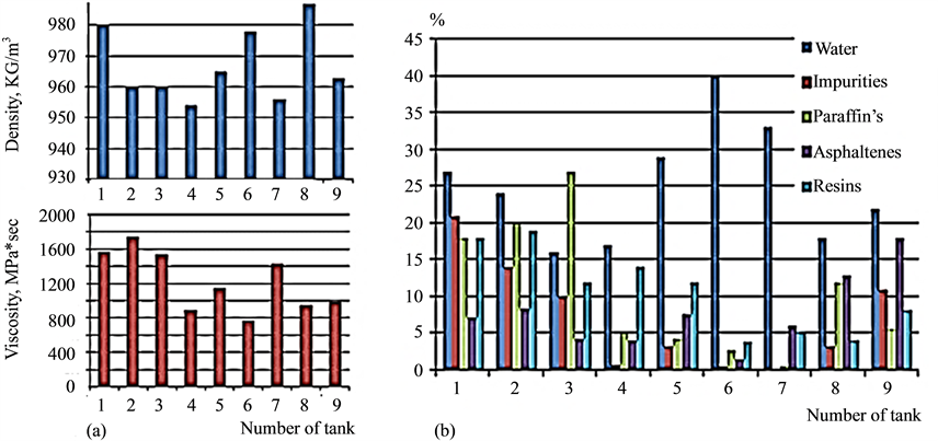
Figure 1. Parameters (a) and content (b) of crude oil sludge in different storage tanks.

Figure 2. Types of sludge layers in storage tank. Layer 1―emulsion “water in oil”; Layer 2―emulsion “oil in water”, medium layer; Layer 3―mineralized water; Layer 4―bottom sludge (solid or of very high viscosity).
 (a) (b) (c)
Figure 3. Schematic design of FR (a) and IFR tanks (b) and photo of internal part of dome tank.
IFR (Internal Floating Roof) tanks are used for liquids with low flash-points (e.g. ATF, MS, gasoline, and ethanol). These tanks are cone roof tanks with a floating roof inside which travels up and down along with the liquid level. This floating roof traps the vapor from low flash-point fuels. Floating roofs are mechanically supported with legs or cables on which they can rest in a maintenance position. EFR (External Floating Roof) tanks do not have a fixed roof (it is open to the ambient environment) and has a floating roof only. Medium flash point liquids such as naphtha, kerosene, diesel, crude oil etc. are stored in these tanks. Figure 3(c). More detail classification of tanks on refineries one can find in [4] .
Storage tanks have different dimensions and capacity. The typical diameters can range from 25 m up to 120 meters and heights up to 22 meters. One of the biggest storage FR tank is shown in Figure 4.
4. Methods and Tools for Sludge Inspection
Currently there are four technologies that can provide sludge inspection and profiling:
1) Manual probing (weighted gauge tape);
2) Measuring density and viscosity versus depth;
3) Acoustic profiling;
4) Infrared thermography.
The first three methods are contact technologies because they require immersion of a device into the oil. Infrared technology is a noncontact technology, because it is measuring the temperature gradient of the outside of the tank shell.
The first three technologies require the device to be inserted thru the roof of the tank and that these entry points are available in suitable quantity and locations for best results. This requirement cannot always be met by

Figure 4. One of the biggest storage FR tank with a capacity 100,000 cubic meters (Northwestern China’s Xinjiang Uygur Autonomous Region).
the tank roof design. Practically they can be used only for storage tanks with external floating roof (EFR tanks), some fixed roof (FR) and in very rare cases in IFR tanks. At the same time, infrared thermography has no restrictions in terms of the type of tank design. These are the main differences of the available technologies and the suitability of their use is determined.
5. Principles of Operation
5.1. Manual Probing
The manual probe presents a small cylindrical sinker fixed on metal tape ruler into the tank. During lowering into the oil the tape undergoes some tension and at the moment of contact with the bottom sludge the tension weakens. This moment is noted by the operator by measuring the length of the tape. Knowing the level of oil and the start point then the height of the sludge can be determined. These measurements are repeated in several entry points and with this data it is possible to use some method of approximation to build a 3D surface of sludge and to then calculate its volume. The simplicity of this method is obvious
5.2. Densitometer & Viscometer Probe
The application of this tool is the same―immersion into the oil thru a roof entry point. The device can log density and viscosity measurements of the tank product with high resolution and accuracy. The data stored in non- volatile local memory and then can be processed. The main advantages of such a device is the ability to obtain detailed information about all the intermediate layers, and often about the type of bottom sludge, as it is the top layer that may have a slightly lower viscosity and density than the lower layer. This tool can detect all layers presented in Figure 2.
5.3. Acoustic Profiler
The acoustic profiler is bathymetric multi-beam sonar for mapping of ocean bottom, adapted for use in crude oil. Typically in such profilers phased arrays used with active acoustic radiation elements made in the form of a Mill’s cross, two-row interference arrays and two-dimensional matrix arrays [5] [6] . The main advantage of such acoustic profilers is the high accuracy of the measurement of the sludge surface, which is usually measured in hundreds of thousands of points and with high speed. For example, for light oil and a tank with a diameter of about 60 meters only one entry point is required. Note that installation time of such a profiler is 3 - 5X more than the time required for data acquisition. As acoustic profiling is carried out in a closed steel volume the acoustic performance is significantly affected by reverberation in the tank. This is caused by various metal structures located in the tank including walls, internal tank temperature gradients which affect the speed of sound, and several other factors that can create different artifacts and distort data. The data post processing includes different custom post-processing algorithms to eliminate these unwanted effects.
5.4. Infrared Thermography Survey of Sludge
Thermography is a type of infrared imaging. Since infrared radiation is emitted by all objects according to the black body radiation law based on their temperature then thermography makes it possible to see some environments with or without visible light illumination. The amount of emitted radiation increases with temperature and thermography can image these temperature variations. Heat transfer occurs differently in gases, liquids and solids due to different thermal capacities and ways of heat transfer thru different materials [7] [8] . For example in water the temperature increase occurs much more slowly than in gas because water has a higher thermal capacity. Fluids and solids have often similar thermal capacities but different manner of heat transfer. Heat transfer in liquids occurs via convection and in solids―via conduction and at appropriate conditions it is possible to detect sludge levels. Let us consider the simplest tank design, and for simplicity let us suggest that water is absent (Figure 5).
Oil and sludge have different coefficients of thermal conductivity, TC, because sludge can contain about 60% - 70% of oil + sand + different impurities and so on. It is these additives that lead to a difference in thermal conductivity. For example, oil has TCoil = 0.14 W/mK0, but sludge which is in general the mixture of sand (TCsand = 0.03) and paraffin’s (TCparaffin’s = 0.11). Therefore the TCsludge will be less than TCoil. This difference is small but nevertheless it can be detected. Steel tanks walls have significantly higher thermal conductivity, TSsteel = 65 - 75 W/mK0. That means that the temperature gradient of the outside tank wall will be different depending on whether it is contacted by sludge or oil. If we make an infrared image of some part of the tank wall then we can see the different temperatures marked by different colors which characterize partial oil or sludge. Taking infrared pictures of the entire wall surface, we can thus determine the border between oil and sludge layers and estimate (measure) the height distribution of sludge near the walls of the tank.
6. Examples
6.1. Measurements of Sludge Based on Data of Density and Viscosity
ITS present below an example of sludge inspection based on density and viscosity data. ITS used a digital portable submersible density & viscosity meter (Figure 6), with some arrangements to deploy it into the tank thru an opening after removing a supporting leg on the EFR tank roof. The tank data is presented in Table 1.

Figure 5. Simplest thermography case.

Figure 6. Density & Viscosity Meter “ViscoDens VDM-250.2 and its installation.
The arrangements of supporting legs are shown in Figure 7(a) and resulted sludge distribution is presented in Figure 7(b) and Figure 7(c).
The color key to Figure 6 is shown in Table 2.
The intermediate layers between oil and sludge are reliably detected. A section view is presented in Figure 8. The measured volume of sludge was V = 2026 m3. The sludge distribution is not uniform due to the flowing product from the inlet and outlet pipes.

Table 1. Tank data.
Table 2. Key to Figure 6.

Figure 7. (a) Arrangements of supporting legs; (b) 2D sludge distribution; (c) 3D Sludge distribution (Courtesy of ITS Asia Pacific Pte Ltd.).
6.2. Measuring of Sludge Based on Thermography Data
For infrared thermography ITS used the IR camera Fluke VT04A Visual IR Thermometer (Fluke Corporation, USA) with applied software Smart View 3.6. ITS have developed additional special software to process thermography images and a methodology for data acquisition. The main feature of this additional software is the selection of the proper range to the tank wall, software to process IR images to detect weak borders in the images with poor color contrast, extraction of this border with automatic estimation of heights, elimination of parallax of images due to the curvature of the tank walls, elimination of large-scale errors and the unification of all individual images into a single image, located along the perimeter of the tank. The last procedure is the approximation of the 3D sludge surface and calculation of the sludge volume. One example of a processed infrared image is presented in Figure 9.
Some images of measured sludge heights and the result of approximation of the 3D sludge surface are presented in Figure 10.
Due to high sensitivity of thermography intermediate layers can be reliably detected. Initial infrared image of the part of wall tank is presented in Figure 11.
Next, Figure 12 demonstrates an arrangement of all detected layers near walls for two tanks with diameter 30 meters.
Reconstructed 3D images of all layers for two tanks (D = 30 meters) are presented in Figure 13.
6.3. Acoustic Profiling of Sludge
Peculiarities of Acoustic profiling of sludge one can find in our paper [6] .
7. Accuracy of Sludge Measurements
Evaluation of the accuracy of measured sludge volume and its 3D surface is rather complicated problem that is

Figure 8. Sections of transient layers (Courtesy of ITS Asia Pacific Pte Ltd.).

Figure 9. Thermography image of part of storage tank with diameter 60 meters. This is a combination of 8 corrected snapshots of IR images connected together. No uniform distribution of sludge is clearly seen (dark blue). The laydowns in sludge profile are due to work of outlet and inlet pipes. Maximum height of sludge is 2 meters (Courtesy of ITS Asia Pacific Pte Ltd.).

Figure 10. Storage tank of 40 meters. Heights of sludge and surface of sludge after approximation (6* scale) V = 1920 m3 ± 250 m3, volume of sludge is 1920 cub meters (Courtesy of ITS Asia Pacific Pte Ltd.).

Figure 11. Snapshot of thermography image of part of tank wall with imposed grid. Intermediate liquid layer is clearly seen (Courtesy of ITS Asia Pacific Pte Ltd.).

Figure 12. Arrangement of layers (Courtesy of ITS Asia Pacific Pte Ltd.).
little discussed in the literature. The main question is “what accuracy is needed”? It is clear that accuracy determines the general cost of tank cleaning and the expenses associated with cleaning: mobilization, type of equipment, cleaning method, time, number of operators, demobilization etc. Then this cost is strongly dependent on the general arrangement of the tank, their geographical location, climate conditions and so on. The level of detail documentation that customer can afford is very important too. For example, when using contact methods, the drawings of roof leg supports for immersion tools need to be presented to the cleaning company.
7.1. Accuracy of Acoustic Profiling
General principle of acoustic profiling is presented in Figure 14.
Beamforming scheme of profiler creates afan of horizontal beams and usually one steering vertical beam. Let’s consider one illuminated area (read spot) and from this area we got the reflected signal. The square of illuminated area depends on directivity of horizontal and vertical beams. The inclination distance R1 is easy to estimate, because after processing we know time delay τ1 of reflecting signal.

Figure 13. 3D Reconstructed Images of sludge and intermediate layers for two tanks (Courtesy of ITS Asia Pacific Pte Ltd.).

Figure 14. General principle of acoustic profiling.
 (1)
(1)
Because we know the vertical steering angle φ1 we can calculate ho as ho = R1sinφ1 and required height of sludge h1
 (2)
(2)
Acting similarly for all scanning horizontal and vertical angles we define all heights of a surface h(x, y). The result of such measurements is the cloud of points h(x, y) which describes the sludge surface in a discrete form. The form of one point can be conditionally presented as “rod, which volume is equal to
 (3)
(3)
Total volume of sludge will be the sum of (3)
 (4)
(4)
Many manufacturers of acoustic profiling tools say that the error of estimated sludge volume is no more that ±5%. However, it has never been reported in what conditions, this accuracy is observed. If this value “±5%” is a hardware accuracy it means that the tool has very modest performance. Certainly manufacturers understand this and they announce stated error ±5% as some average operation value. But the real accuracy of acoustic profiling in closed reverberation areas as crude oil tanks is a very complex subject and it requires a special investigation.
Let us present some examples to illustrate only part of this problem. In this case, we assume that the hardware accuracy of profiler is very high; in other words, the arrays have very narrow beams, low level of side-field, transmit level is sufficient to provide high input signal/noise ratio and other features that characterize the high quality of such an acoustic bathymetry tool. Let us take an EFR tank with diameter D = 50 m with crude oil which level is Hoil = 10 m. So the volume of crude is Vcr = πR2Hoil = 3.14 * 252 * 10 = 19625 m3. Now let us propose that acoustic profiling with ±5% accuracy estimated sludge volume about Vsl = 1000 m3 ± 50 m3. An acoustic profiler cannot measure the thickness of intermediate sludge layers which are always present in crude. Let us take its thickness as 10 cm (Figure 7). This layer thickness of 10 cm means an additional sludge volume Vadd = 3.14 * 625 * 0.1 = 196 m3 (!). Therefore the real accuracy of acoustic profiling will range from 14.6% up to 24.5% (!) or 3 - 5X worse. Therefore, the stated accuracy ±5% of the acoustic profiling should be treated with caution.
Another case is related to sound speed in crude. The accurate value of sound speed determines all inclination ranges to the points of the reflected probe signal and therefore the local heights of sludge. It is possible to say that knowledge of correct sound speed is a determining factor for accuracy. Sound speed can be measured in different ways: by reflection of the probe pulse from the tank wall or bottom or by using a special HF sound speed meter. Generally the error of speed of sound determines the error of measured sludge volume.
 (5)
(5)
If we measure sound speed with an error ±5% the error of measured volume will be the same. Formula for sound speed in crude can be written as
 (6)
(6)
where
 (7)
(7)
Because density of oil is known with a very high accuracy the errors of sound speed play major role. The problem arises when sound speed profile can be not uniform on the depth of tank which is sometimes typical for large tanks located in geographic areas with sharp fluctuations in day and night temperatures. Below there is one of such example of measured temperature in oil tank with API = 36 on different depths and calculated sound speed (Figure 15).
The presented temperature distribution will inevitably create refraction of sound rays, which lead to two main effects. Firstly the shape of the sludge surface will be distorted because its reflecting points will not be visible in those locations where they actually exist. Secondly, errors in vertical angle of steering relative to the tank bottom will give errors in measured heights and result in significant errors of estimated volume. For a given sound profile for example, the errors of heights can range from 5 cm up to 65 cm depending on the angle of vertical steering. The use of acoustic profiling should be accompanied by measurements of the vertical temperature profile, especially for large diameter tanks. In the presence of significant refraction of sound rays the software for surface and volume calculations should include calculations of the beam paths for the introduction of appropriate corrections
7.2. Accuracy of Contact Point Measurements of Density & Viscosity
7.2.1. Modelling
It is understood that the accuracy of contact measurement directly depends on the number of possible entry points. And for general cases, this statement is true. However, the use of a large number of entries is always limited for various reasons. Therefore it is of interest to understand what number of entries we need to obtain a predetermined error of sludge volume and real shape of its surface. As a rule the sludge surface has a random character so it is best to characterize the shape of the surface with statistical parameters and in particular by spatial correlation radius of irregular heights, Rh. First of all let us consider some results of modelling. We have selected a tank with diameter 50 meters and 52 supporting legs, see Figure 16.

Figure 15. Vertical profile of sound speed in a storage tank.
Initial sludge distribution in the tank was defined randomly with the following law:
 (8)
(8)
Here, hmin is the minimal sludge level, Δh is the sludge level deviation amplitude, rnd―random number between 0 and 1 for each position x, y. In order to obtain different types of sludge (smooth or “rough”, low or high level etc.) different model parameters hmin, Δh and the correlation of the h(x, y) distribution defined as Rcor were chosen. True volume of sludge was calculated as

Typical model distributions are shown in Figures 17-19.

Figure 16. Arrangement of supporting legs.

Figure 17. Regular sludge distribution. hmin = 1 m, Δh = 1 m, Rcor = 5 m, V0 = 2925 m3.
The next data contain simulation results for an incomplete set of measurement points. Cases with 5, 10 and 15 missing leg points (of 52) were investigated for 3 basic distribution models (“regular”, “low-level” and “high- level”) with 5 interpolation models (triangular linear, nearest, Gaussian RBF, multiquadric RBF, thin plate RBF). The results are presented in graphs of Figure 20.

Figure 18. Low-level distribution with following parameters (shown magnified): hmin = 0 m, Δh = 2 m, Rcor = 5 m, V0 = 1866.5 m3.

Figure 19. High-level smooth distribution with following parameters (shown magnified): hmin = 1.5 m. Δh = 1.5 m, Rcor = 7 m. Vo = 4365.7 m3.

Figure 20. Errors of estimated volume versus missing point for three models of sludge distribution, for different types of approximation of the surface (a) Regular distribution, (b) Low-level distribution, and (c) High-level distribution (Courtesy of ITS Asia Pacific Pte Ltd.).
7.2.2. Experimental Results
The EFR tank had more than 52 supporting legs, but only 31 legs were available and their arrangement is presented in Figure 21.
tank diameter 65900 mm;
tank bottom details: cone up, center height 275 mm;
level of oil 14050 mm.
These are some results from the processing of data for the tank in Figure 22. All measurements were made with a digital Density & Viscosity Meter.
The final results are presented in Table 3.
The comparison of simulated data and experimental data is presented in Figure 23.
We can see that the experimental data is in very good agreement with the theoretical curve. This high degree of correlation supports the validity of the mathematical method. The theoretical relationship can be used for pre-planning of the contact measurement method of sludge in any crude oil tanks with a sufficient number of entry points. To obtain the value of the error of the sludge volume in the range of 8% - 10% the required number of entry points should be no more than 20 - 25.
7.3. Accuracy of Thermography Imaging of Sludge Distribution
Physical data obtained by IR camera corresponds to the distribution of sludge heights along the tank walls but with no information about the inner tank sludge data points. Therefore, we can use only the tank wall data for further processing. The initial conclusion is that this method will have the worst accuracy in comparison with the other discussed methods. However, such a conclusion is quite hasty and not quite accurate. Remember, that when applying contact measurements at different entry points the 20 readings were sufficient to get an accuracy of about 12% - 15% for the sludge volume. Using an IR camera we can get a significantly higher number of readings and a practically arbitrary amount of them, this is the first point. The second point is a random sludge distribution which is rather uniform in the average if tank mixers are not used. That means that from statistical

Figure 21. Arrangement of available entry points. Key: Available entry points (blue dots) distribution. Green dot―reference point, White dot―centre point, Small red triangle―inlet pipe 16”, Big red triangle―inlet pipe 32”. Small yellow triangle―outlet pipe 16”.

Figure 22. 3D Images of sludge distribution with missing legs arrangement of available entry points. Key: Available entry points (blue dots) distribution. Green dot―reference point, White dot―centre point, Small red triangle―inlet pipe 16”, Big red triangle―inlet pipe 32”. Small yellow triangle―outlet pipe 16” (Courtesy of ITS Asia Pacific Pte Ltd.).

Figure 23. Comparison of simulated data and experimental data (Courtesy of ITS Asia Pacific Pte Ltd.).
point of view the statistical parameters of sludge heights inside the tank should be similar to the statistical parameters of height distribution along the wall. Therefore if the radius of space correlation of sludge irregularities is rather small it can be argued with a high level of probability that the statistics of sludge heights inside the tank will be similar to the statistics of sludge heights near the walls. In this case, we certainly cannot reproduce the true surface of sludge dirt, but the error of its volume can be significantly reduced.
Modelling
For simulation we used the same methodology described in Section 7.2.1, excluded all data inside the tank, and used only the values of “walls” heights (Figure 24).
We simulated three types of sludge surface: “low-level” distribution with average level of 0.8 m with deviation ±0.3 m, “Regular” distribution with average level of 2.5 m with deviation ±0.5 and sludge surface formed with a mixer stream. For each type of sludge the surface was generated 30 times. The results are presented in Figures 25-27.
In the case of infrared sludge profile registration both profile reconstruction and volume estimation can be accomplished but with rather high errors (25% - 40%). It can be seen from Tables 1-3 that the estimated values of sludge volume are underestimated for all considered cases. For cleaning purposes it leads to a simple correction algorithm: estimated values based on IR data should be increased by 30% - 35% depending on the sludge profile uniformity obtained on the IR images. Note that there is another way of decreasing an error of volume based on IR data which will be described later in the next article.
Table 3. Final results.

Figure 24. Simulated profile of sludge and height profile near the tank wall.

Figure 25. Calculated volumes for low level sludge distribution (Courtesy of ITS Asia Pacific Pte Ltd.).

Figure 26. Calculated volumes for for regular distribution of sludge (Courtesy of ITS Asia Pacific Pte Ltd.).

Figure 27. Calculated volumes for sludge with mixed stream (Courtesy of ITS Asia Pacific Pte Ltd.).
8. Discussion: Advantages and Disadvantages of Different Methods of Sludge Estimation
The use of the discussed methods for estimating sludge volume depends on several factors. In the table below we have tried to consider all the pros and cons of the considered methods both in terms of their technical and operational features, leaving the choice of method to the user.
Technical factors as shown in Table 4 include hardware accuracy of the instrument, its complexity, reliability and weight. The ranges of operational requirements are much wider as shown in Table 5. These include the type of oil storage tank, available number of entry points, ability to work in all types of oil, the time of installation of the device and the time of inspection, presence of operators on the roof of the tank, and the number of such personnel, the ability to detect the intermediate layers and the need to stop the tank operations during the inspection.
9. Conclusions
This research shows that there is no single universal method for estimating the volume of sludge and its spatial distribution that combines the highest accuracy and the ability to be performed on any tank.
Acoustic profiling typically allows estimation of the distributed sludge surface with a high accuracy for tanks with external floating roofs. However, the accuracy of the surface and its volume requires additional information and rather complex post-processing. This situation is analogous to ocean floor acoustic bathymetry, where the raw data are received fast enough, but the construction of a true bottom image requires rather lengthy processing of the primary raw data. A significant limitation of the acoustic profiling techniques is the inability to use them in oil with high viscosity, i.e. in the heavy and extra-heavy oil.
Table 4. Technical factors.
Table 5. Operational factors.
Using contact devices that directly measure the density and viscosity of the product in the tanks gives the most information since they can detect all the layers, including water. However, to generate a surface, it is only possible in tanks with external floating roofs with a sufficient number of entry points.
Infrared thermography is the most convenient and expedient method of inspection for oil storage tanks, and most importantly, this is a noncontact method. Although it is less accurate than the contact methods, it can be used for tanks of any types, and for all types of petroleum or its products. From this point of view, the thermography method is the most flexible and convenient. This means that it can easily be included as part of a refinery monitoring plan for sludge accumulation in tanks.
Various types of oil storage tanks are located in all refineries. Therefore, the most comprehensive solution is to use the three considered methods where applicable.
Acknowledgements
We wish to thank the entire staff of the ITS Asia Pacific Pte Ltd. for their great help and field work in the preparation of the initial data that forms the basis of this article.
References
- Velghe, I., et al. (2013) Study of the Pyrolysis of Sludge and Sludge/Disposal Filter Cake Mix for the Production of Value Added Products. Bioresource Technology, 134, 1-9. http://dx.doi.org/10.1016/j.biortech.2013.02.030
- Lima, C.S., et al. (2014) Analysis of Petroleum Oily Sludge Produced from Water-Oil Separator. Revista Virtual de Química, 6, 1160-1171.
- Bokovikova, T.N., Shperber, E.R., Shperber, D.R. and Marchenko, L.A. (2014) Management Oil Waste of Primary Oil Refining. Letters in International Scientific Journal for Alternative Energy and Ecology, 1, 27-36.
- Storage Tank. http://en.wikipedia.org/wiki/Storage_tank
- T-Type Sludge Mapping System. http://www.oceanscan.net/c-Products
- Monteiro, M., Svet, V. and Sandilands, D. (2014) The Features of Acoustic Bathymetry of Sludge in Oil Storage Tanks. Open Journal of Acoustics, 4, 39-54.
- Hooyberghs, H. (2013) “Pictures” the Emissions of Storage Tanks with the Use of Infrared Cameras. 6th Annual Aboveground Storage Tank Conference & Trade Show Houston, Houston, 19 September 2013, 16-21.
- Venkoparao, V. and Sai, B. (2013) Method and Apparatus for Automatic Sediment or Sludge Detection, Monitoring, and Inspection in Oil Storage and Other Facilities. US Patent No. 8452046.