Advances in Remote Sensing
Vol.2 No.4(2013), Article ID:40774,15 pages DOI:10.4236/ars.2013.24033
Validation of High-Density Airborne LiDAR-Based Feature Extraction Using Very High Resolution Optical Remote Sensing Data
1Earth System Sciences Organization, National Centre for Antarctic and Ocean Research (NCAOR), Ministry of Earth Sciences, Government of India, Headland Sada, Goa, India
2Centre for Environmental Planning & Technology (CEPT) University, Ahmedabad, India
Email: *shridhar.jawak@gmail.com; shridhar.jawak@ncaor.gov.in
Copyright © 2013 Shridhar D. Jawak et al. This is an open access article distributed under the Creative Commons Attribution License, which permits unrestricted use, distribution, and reproduction in any medium, provided the original work is properly cited.
Received October 15, 2013; revised November 11, 2013; accepted November 15, 2013
Keywords: LiDAR; WorldView-2; feature extraction
ABSTRACT
This work uses the canopy height model (CHM) based workflow for individual tree crown delineation from LiDAR point cloud data in an urban environment and evaluates its accuracy by using very high-resolution PAN (spatial) and 8-band WorldView-2 imagery. LiDAR point cloud data were used to detect tree features by classifying point elevation values. The workflow includes resampling of LiDAR point cloud to generate a raster surface or digital terrain model, generation of hill-shade image and intensity image, extraction of digital surface model, generation of bare earth digital elevation model and extraction of tree features. Scene dependent extraction criteria were employed to improve the tree feature extraction. LiDAR-based refining/filtering techniques used for bare earth layer extraction were crucial for improving the subsequent tree feature extraction. The PAN-sharpened WV-2 image (with 0.5 m spatial resolution) used to assess the accuracy of LiDAR-based tree features provided an accuracy of 98%. Based on these inferences, we conclude that the LiDAR-based tree feature extraction is a potential application which can be used for understanding vegetation characterization in urban setup.
1. Introduction
Trees in metro and cities contribute significantly to urban environmental quality. However, techniques are used to assess urban forest resource and their possible impact on the regional scale is less explored. To better understand the urban forest resource and its numerous values, surveying and mapping individual tree structures help in the advancement of the understanding of the urban forest structures, improve urban forest policies, offer data for prospective inclusion of trees in environmental regulation studies, and determine how urban trees affect the urban environment and accordingly enhance environmental quality in urban areas for human health.
Light detection and ranging (LiDAR) is an active remote sensing technology that evaluates properties of reflected light to determine range to a remote object [1]. Airborne LiDAR is capable of providing highly accurate measurements of vertical features with single pulse, multiple pulses, or full waveform. However, its usage is currently limited because of its high acquisition cost. In LiDAR remote sensing, the range to remote object is estimated by computing the time delay between broadcast of a laser pulse and recognition of the reflected signal [2]. LiDAR technology is being progressively more practiced in ecology, forestry, geomorphology, seismology, environmental research and remote sensing because of its capability to produce three-dimensional (3D) point data with high spatial resolution and better accuracy [1, 3-8]. LiDAR systems coupled with accurate positioning and orientation systems can obtain precise 3D measurements of earth surface in the form of point cloud data by using high sampling densities [9]. LiDAR point cloud data filtration and interpolation has been a field of research for last many years and thousands of methods have been introduced for this process. In case of LiDAR filtration and interpolation, two assumptions are significant: 1) earth surface is continuous and smooth, and 2) the neighboring point data are correlated. LiDAR interpolation methods are broadly classified into two categories: 1) deterministic methods, and 2) geostatistical methods. Deterministic methods assume that each input LiDAR point has a local weight with the spatial distance [10], whereas the geostatistical methods are based on the spatial distance as well as the spatial correlation for interpolating the LiDAR point data [11]. Inverse distance weighted (IDW) method is based on linear weighted arrangement of set of sample points, where higher weight is assigned to the points which are spatially closer to the sample point [10]. Hence, IDW performs better for densely distributed LiDAR data where cloud points are closely and evenly spaced [12]. Spline interpolation employs a numerical function to approximate the interpolated values that diminish the large curvature of the surface considering all the data points [13]. On the other hand, Krigging interpolation takes into account the spatial correlation between LiDAR data points for generating continuous surface. Moreover, the Kriging interpolation is based on mutual spatial distance between the LiDAR data points, and its efficiency is verified by semivariogram [11,14,15].
Individual tree feature extraction has significant applications in forestry, ecology, and environmental studies [16-18]. The structural characteristics of individual tree feature such as tree height, crown diameter, canopy based height, diameter at breast height (DBH), biomass, and species type can be derived after an accurate extraction of individual tree [17,19,20]. The traditional methods for extracting individual tree features include field inventory and aerial photograph interpretation. However, traditional methods have certain limitations such as requirement of intensive field work and financial implications which can be overcome by using airborne LiDAR [21] and very high resolution satellite images. Field inventories are generally labour-intensive, time-consuming, and limited by geographical accessibility [7]; optical aerial photography does not directly provide 3D tree structure information [16]. The ground-based LiDAR is capable of capturing detailed 3D measurement of tree structure; however, it is less effective for large geographical extent.
LiDAR has been widely applied in forestry [22-29], and it is found to be useful in mapping individual trees in complex forests [8,16-18,26]. Research on exploiting LiDAR point cloud data to evaluate vegetation structures has been progressed from a forest scale to individual tree level [30]. This is evidently encouraged by the developments in LiDAR technology, resulting in higher pulse rates and increased LiDAR point densities. Therefore, the semiautomatic extraction of single tree (delineation) has become a fundamental approach in forestry research [31]. Computing tree attributes at high spatial scales is essential to monitor terrestrial natural resources [32]. However, not many studies have focused on individual tree level feature extraction [29]. One of the main challenges of this research is result validation and accuracy assessment for individual extracted tree measurements, where detailed field inventory and/or very high resolution satellite image are/is necessary. The high spatial density LiDAR point cloud data noticeably reveal the structure of individual trees, and hence provide better prospect for more accurate tree feature extraction and vegetation structure parameters. The high density LiDAR has been successfully used to demarcate the whole structure of individual tree [33-36]. There are numerous methods proposed to demarcate individual trees by using airborne LiDAR point cloud data. Popescu and Wynne [26] employed a local maximum filtering method to extract individual trees. Tiede et al. [37] practiced a similar local maximum filtering method to recognize tree tops and developed a region growing algorithm to extract tree features. Chen et al. [16] proposed a watershed segmentation to isolate individual trees, where the tree tops extracted by local maxima were used as markers to improve the accuracy. Koch et al. [18] extracted tree features by synergetic usage of pouring algorithm and knowledge based assumptions on the structure of trees. Korpela et al. [19] used a multi-scale template matching approach for tree feature extraction using elliptical templates to represent tree models. Falkowski et al. [38] proposed the spatial wavelet analysis to semiautomatically verify the spatial location, height, and crown diameter of individual tree features from LiDAR point cloud data. These algorithms extract individual tree features by using the LiDAR derived canopy height model (CHM). CHM is a raster image interpolated from LiDAR cloud points indicating the top of the vegetation canopy. Tree detection and tree crown delineation from Airborne LiDAR have been mostly utilizing the CHM. However, CHM can have inherent errors and uncertainties, e.g., spatial error introduced during the interpolation from the point cloud to raster [39], which may reduce the accuracy of tree feature extraction. Therefore, new methods to delineate individual tree features from the LiDAR point cloud necessitate development and validation. Morsdorf et al. [40] employed the k-mean clustering algorithm to delineate individual tree features from the point cloud, but their accuracy depended on seed points extracted from the local maxima of a digital surface model. Lee et al. [41] developed an adaptive clustering approach to segmenting individual trees in pine forests from the raw LiDAR point cloud data. This method is based on the concept of watershed segmentation and it requires adequate training data for supervised learning.
In this study, we used a method for individual tree delineation based on canopy height model (CHM) from the high resolution airborne LiDAR point cloud data. To investigate the algorithm’s effectiveness in extracting individual trees, we used very high resolution remote sensing data from WorldView-2 satellite. This study aims to assess the accuracy of individual tree extraction while using LiDAR by visual interpretation of trees onto very high resolution WorldView-2 image. Figure 1 shows LiDAR point cloud.
2. Study Area and Geospatial Data
2.1. Study Area and Environment
In order to investigate and illustrate the effectiveness of LiDAR based tree feature extraction, we selected the part of San Francisco city, California, United States of America (37˚44"30'N, 122˚31"30'W and 37˚41"30'N, 122˚ 20"30'W), as a test scene. San Francisco is situated on the West Coast of the USA at the north ending of the San Francisco Peninsula and comprises of significant extension of the Pacific Ocean and San Francisco Bay within its margins. Several islands—Treasure Island, Yerba Buena Island, Alameda Island, Farallon Island, Red Rock Island, and Angel Island—are essential parts of the city. The mainland area within the city constitutes roughly 600 km2. There are more than 50 hills within city boundaries. There are more than 220 parks maintained in the San Francisco by Recreation & Parks Department, containing thousands of native trees and plants. QuickBird satellite imagery of the study area captured on 11th November 2007 is shown in Figure 2.
2.2. Urban Forest Structure of San Francisco
An analysis of trees reveals that the urban forest of San Francisco has an approximately 669,000 trees [42]. Trees cover about 11.9% of San Francisco; shrubs cover 6.9% of the city. Dominant ground cover types include impervious surfaces (excluding buildings) (e.g., driveways, sidewalks, parking lots) (42.5%), buildings (26.1%), and herbaceous (e.g., grass and gardens) (19.3%). Trees having diameters less than 6 in are reported to be 51.4% of the total tree population. The three most common species
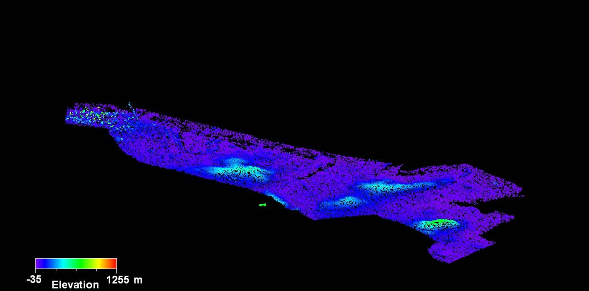
Figure 1. LiDAR based point cloud representation over the extent of study area.
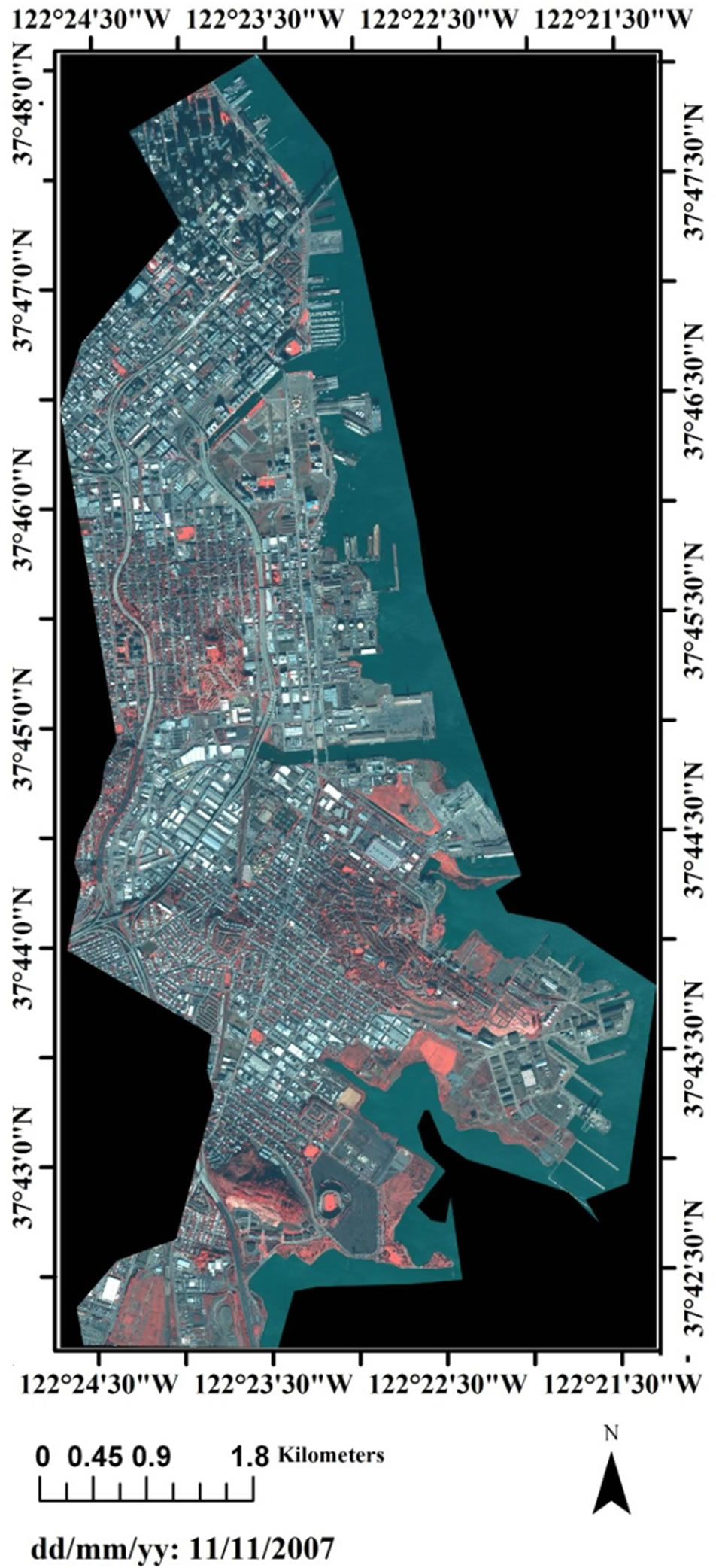
Figure 2. QuickBird PAN-sharpened satellite image over the study area.
in the urban forest are blue gum eucalyptus (15.9%), Monterey pine (8.4%), and Monterey cypress (3.8%) [42]. The highest density of trees is found in the open space (36.9 trees per acre), followed by the institutional land (24.0 trees per acre) and street right of ways (23.7 trees per acre) [42]. San Francisco’s urban forests consist of a mixture of native tree species and exotic tree species. Hence, urban forests often have a tree diversity that is higher than adjacent native landscapes. In San Francisco, about 16% of the trees are from species native to California state. Trees with a native origin outside of North America are mostly from Australia (29.3% of the species) [42].
2.3. Remotely Sensed Data
We used the standard airborne LiDAR data over San Francisco, California, USA, recorded in June 2010. The data was in LASer (LAS) format which is a file format specification for the interchange of 3D point data (x, y, z triplet per point) approved by American Society for Photogrammetry and Remote Sensing (ASPRS) [9]. In addition to airborne LiDAR data, we also used radiometrically-corrected, geo-referenced, orthorectified 16-bit standard level 2 (LV2A) WV-2 multi-sequence datasets, including single band PAN and 8-band MSI images at 46 cm and 185 cm ground sample distance, which were resampled to 50 cm and 200 cm, respectively. The data was provided with tiles of 8-band MSI and single-band PAN images, which were spatially mosaicked to generate a single continuous image for each region. Level 2A of image preprocessing was done by the DigitalGlobe. This preprocessing entails standard ortho-correction using base elevation from a relative coarse resolution DEM, nearest neighbour (NN) resampling method using standard kernel filters and standard radiometric correction procedure. The images which were acquired in nearly cloud-free bright illumination on 9th October 2011 over San Francisco covered a number of buildings, vegetation structures, forest structures, skyscrapers, industrial structures, residential houses, highways, community parks, and private housing (Figure 3). The images were geometrically corrected and georegistered to World Geodetic System (WGS) 1984 datum and the Universal Transverse Mercator (UTM) zone 10N projection. The calibration metadata was used to convert the raw digital numbers to radiance. This information is adequate to assess the potential of airborne LiDAR data for extraction of tree features.
2.4. Reference Data for Accuracy Assessment
The remote sensing (RS) data cannot be used efficiently without ground truth, especially for urban studies. The successful interpretation of RS data requires supplementary field work to understand the small-scale variations that are common in urban land cover. PAN-sharpened WV-2 (0.5 m) supplemented by publicly available GIS maps and historical Google Earth images were used for accuracy analysis. The ground truth datasets used to support tree feature mapping include survey data (http:// www.sftrees.com/), San Francisco's comprehensive urban forest report (available on http://www.nrs.fs.fed.us /pubs/rb/rb_nrs008.pdf), urban forest maps (available on http://urbanforestmap.org/map/), publically available city maps, and historical Google Earth images and maps (Figure 4).
3. Methodology
3.1. Worldview-2 Processing
Preprocessing of the WorldView-2 imagery comprises of
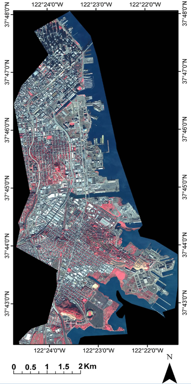
Figure 3. WorldView-2 PAN-sharpened image (50 cm spatial resolution) showing the spatial extent of study area.
four separate steps: 1) data preparation, 2) data fusion, 3) co-registration of WV-2 Pan-sharpened images to the LiDAR data, and 4) shadow compensation using LiDAR based DSM.
3.1.1. Data Preparation
1) Dark pixel subtraction: First, a dark pixel subtraction was performed to reduce the path radiance from each band. The dark object is the minimum digital number (DN) value for more than 1000 pixels over the whole image [43]. The dark objects need to be carefully chosen from the scene; clear water bodies and dark vegetation under shadows are traditionally selected as dark objects [44,45]. Clear water bodies were used as dark objects in our analysis following the literature [46]. The DN values for DOS per band for the WV-2 image are: [11,29,33,36, 39,47,51,81].
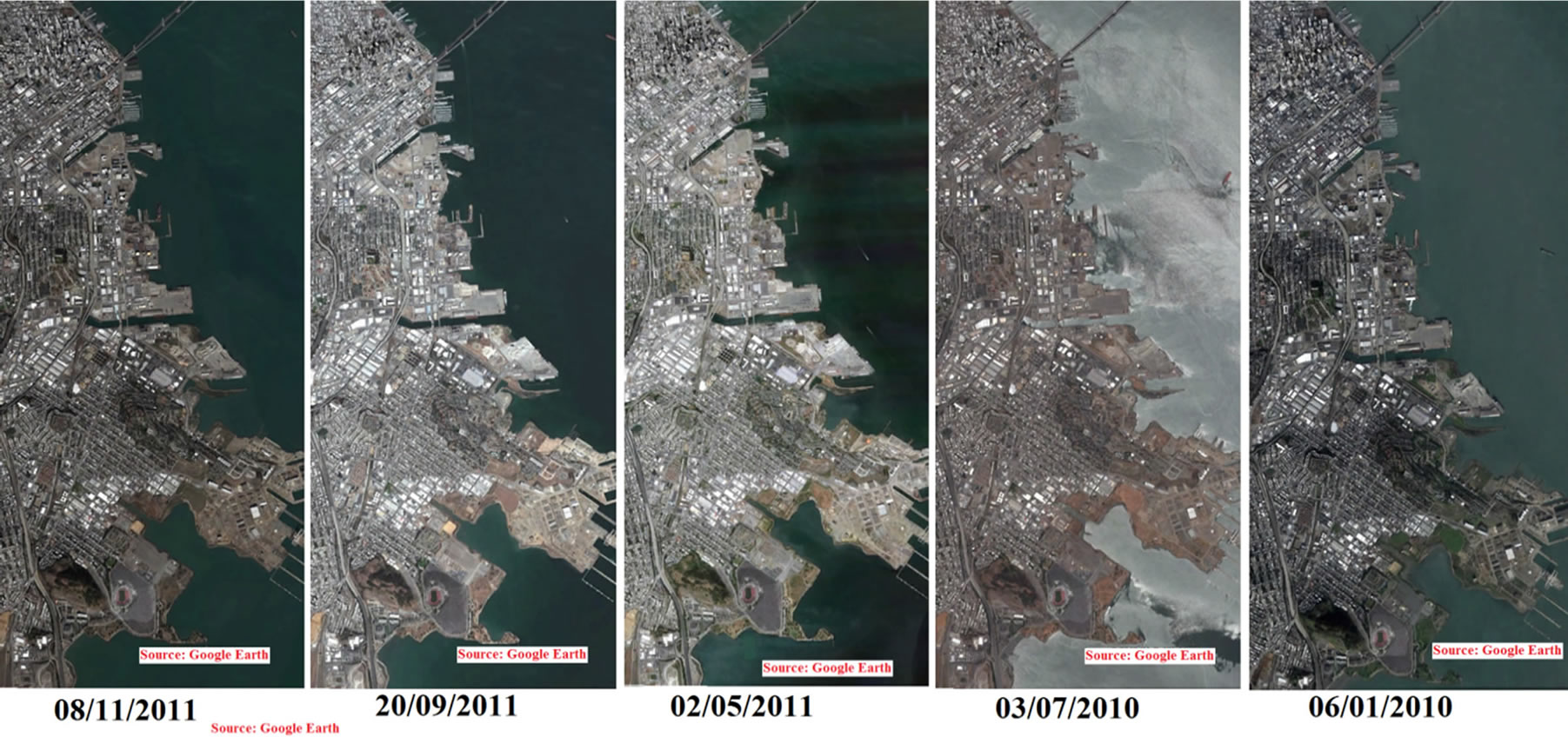
Figure 4. Multitemporal Google Earth images used in present study as a supplementary source for accuracy assessment.
2) Data calibration: Calibration of image spectrometer data necessitates radiometric corrections, which require a function to convert the DN into the at-sensor radiance [47]. The at-sensor radiance was calibrated to minimize atmospheric effects. The calibration method was adapted from literature [48]. The calibration procedure was carried out in two steps: 1) conversion of the raw DN values to at-sensor spectral radiance factors and 2) conversion from spectral radiance to Top-of-Atmosphere (TOA) reflectance.
3.1.2. Data Fusion
In order to provide a detail spatial context to the study, fusion of MS image and PAN image was necessary [49-52]. In the present study, the PAN and MSI were captured at the same time and with the same sensor. Hence, PAN-sharpening was carried out without further registration [53,54]. In order to create an image at 0.50 m resolution [55-57], the multiband image was PANsharpened from a resolution of 2.00 m to 0.50 m by using Hyperspherical Color Sharpening (HCS) fusion method which has been specifically developed for the WV-2 data [58]. Since the HCS resolution merge algorithm requires smoothing filters, we used three filters 3 × 3, 5 × 5, and 7 × 7 to yield three PAN-sharpened images. The image with the least spatial artifacts was selected by visual interpretation. Finally, the HCS-sharpened image with the dimension 5 × 5 convolution filter was selected for further analysis.
3.1.3. Co-Registration
The first and possibly most important precursor step of the tree feature extraction process is the precise co-registration between all datasets. In fact, neglecting georegistration can lead to false accuracy analysis. The optical WV-2 data and the LiDAR intensity image were coregistered. Co-registration was performed in two steps: 1) geometric correction without ground control points (GCPs) and 2) ortho-rectification using ground control points. The main challenge was to match the resolution of LiDAR intensity image with the resolution of PANsharpened WV-2 image. At first, the WV-2 rational polynomial coefficients model (RPC) was executed in ERDAS Leica Photogrammetry Suite (LPS) using supplementary (.RPB) file. In the second stage, orthorectification was carried out using ERDAS LPS by incorporating well-distributed GCPs. The obtained root mean square error (RMSE) for the WV-2 was estimated to be 0.25 m using more than 10 well-distributed GCPs.
3.1.4. Shadow Compensation Using LiDAR Based DSM
For hilly environments with high geographic relief, local topography may cause cast shadows due to the blocking of direct solar radiation. The optical RS images of these landscapes display reduced values of reflectance for shadowed areas compared to non-shadowed areas with similar surface cover characteristics. Since PAN-sharpened WV-2 image was used for accuracy analysis and visual interpretation, pre-masking of shadowed tree features was necessary. We used the most straightforward method for compensating shadows from imagery by using the digital surface model (DSM) based shadow detection and pre-extraction compensation, following Rau et al. [59] in urban areas, and Giles [60] in mountainous areas. We used the LiDAR-based DSM of San Francisco for shadow compensation. The cast shadow from WV-2 image was computed from aforementioned DSM and the sun elevation information at the time of WV-2 image acquisition. The DSM-based shaded relief map and shadow map (Figure 5) were prepared in order to identify the shadow pixels formed by the topography and low sun angle. It is noted that the region affected by cast shadow was masked for the tree extraction accuracy analysis process. These shadowed trees were manually checked after non-shadowed (open) tree extraction accuracy analysis by visual interpretation using supplementary field datasets coupled with multi-temporal satellite images.
3.2. LiDAR Data Processing
A step by step workflow used in this research is shown in Figure 6. LiDAR-based individual tree feature extraction consists of five main tasks: 1) bare earth digital elevation /terrain (DEM/DTM), DSM, and intensity image generation, 2) building footprint extraction, 3) individual trees/ vegetation/forest extraction using CHM, 4) tree filtering, and 5) accuracy assessment of tree feature extraction. Many different software packages are available to resample LiDAR point clouds into 2-D grids and advanced processing. We utilized Overwatch system’s LIDAR Analyst for ArcGIS, LAStools© software, and QCoherent software LP360 for ArcGIS. Methodology consists of five steps:
3.2.1. Extraction of Bare Earth Digital Elevation/Terrain (DEM/DTM) and Digital Surface Model (DSM)
Conversion of point clouds to uniform raster surfaces or 2D-grids by resampling methods is the first essential step in many LiDAR based applications. Many surface interpolation methods are available in literature for effective rasterization [61]. The choice of cell size affects the quality of 2D-raster models or surfaces generated. We selected a grid size of 50 cm to match the 50 cm resolution of PAN-sharpened WV-2 image and based on average tree diameters interpreted using WV-image. A bare earth DEM/DTM, a DSM and an intensity image were derived from the raw airborne LiDAR data. The DEM/ DTM was generated by triangulating elevation values only from the bare-earth LiDAR points, while the DSM was generated by triangulating elevation only from the first-return LiDAR points (Figure 7). The intensity image was generated by triangulating intensity from the first-return LiDAR points. Surfacing was used to interpolate the ground points and generate the DEM [62]. In this study, the ground points were collected and interpolated using an adaptive triangulated irregular network (TIN) model. We employed TIN interpolation method over IDW and spline, because the LiDAR point cloud data was very dense and spline and IDW method failed to give desired results. TIN approach also considers the density variation between data points. As the study area is urban, this method provided good results when compared to other methods like Kriging which is useful in the areas consisting of diverse features which exhibit high degree of spatial auto-correlation. Bare earth DTM/ DEM extraction is followed by editing or cleaning of that bare earth layer. In most of the cases, bare earth DEM does not represent true ground elevation. Hence, the model was cleaned/ edited to get the most accurate DEM/ DTM possible. After DTM editing, we normalized the LiDAR point cloud data based on DTM in order to reduce the effect of undulating terrain. The normalization step is very significant since the tree filtering algorithm needs to define a reference height for further processing. We normalized the vegetation point cloud values by subtracting the ground points (DEM) from the LiDAR point cloud [41]. A normalized digital surface model (nDSM) or CHM is calculated from the LiDAR data by subtracting the DEM from the DSM. The CHM or the normalized DSM represents the absolute height of all aboveground urban features relative to the ground. After normalization, the elevation value of a point indicates the height from the ground to the point. The above-ground points were used for tree feature and building footprint extraction.
3.2.2. Building Footprint Extraction
The second step of the workflow is to identify building measurements from non-building (mainly vegetation) data to aid tree feature extraction. Building footprint extraction consists of extracting the footprints of buildings in 3D shapefile format along with the attribute table showing the information about each building polygon. This task also consists of editing building footprint layer so as to separate the merged buildings. We employed LiDAR analyst 4.2 for ArcGIS workflow for buiding extraction. The parameters used for building extraction are listed in Table 1-3. The final output map of building feature extraction is shown in Figure 8.
3.2.3. Individual Trees/Vegetation/Forest Extraction
We used the CHM based method for individual tree feature extraction. The individual tree extraction based on this method produces 3D shapefile for extracted tree features. It is generally assumed that the LiDAR points other than the terrain are tree features in the urban areas. The calculation of individual tree height is difficult because it is indistinct where the laser pulse hits and reflects from the tree. A local maximum filtering with variable search window approach was used to detect tree features. In individual tree extraction, first and last return point clouds were used along with the bare earth and building footprint models discussed above. While
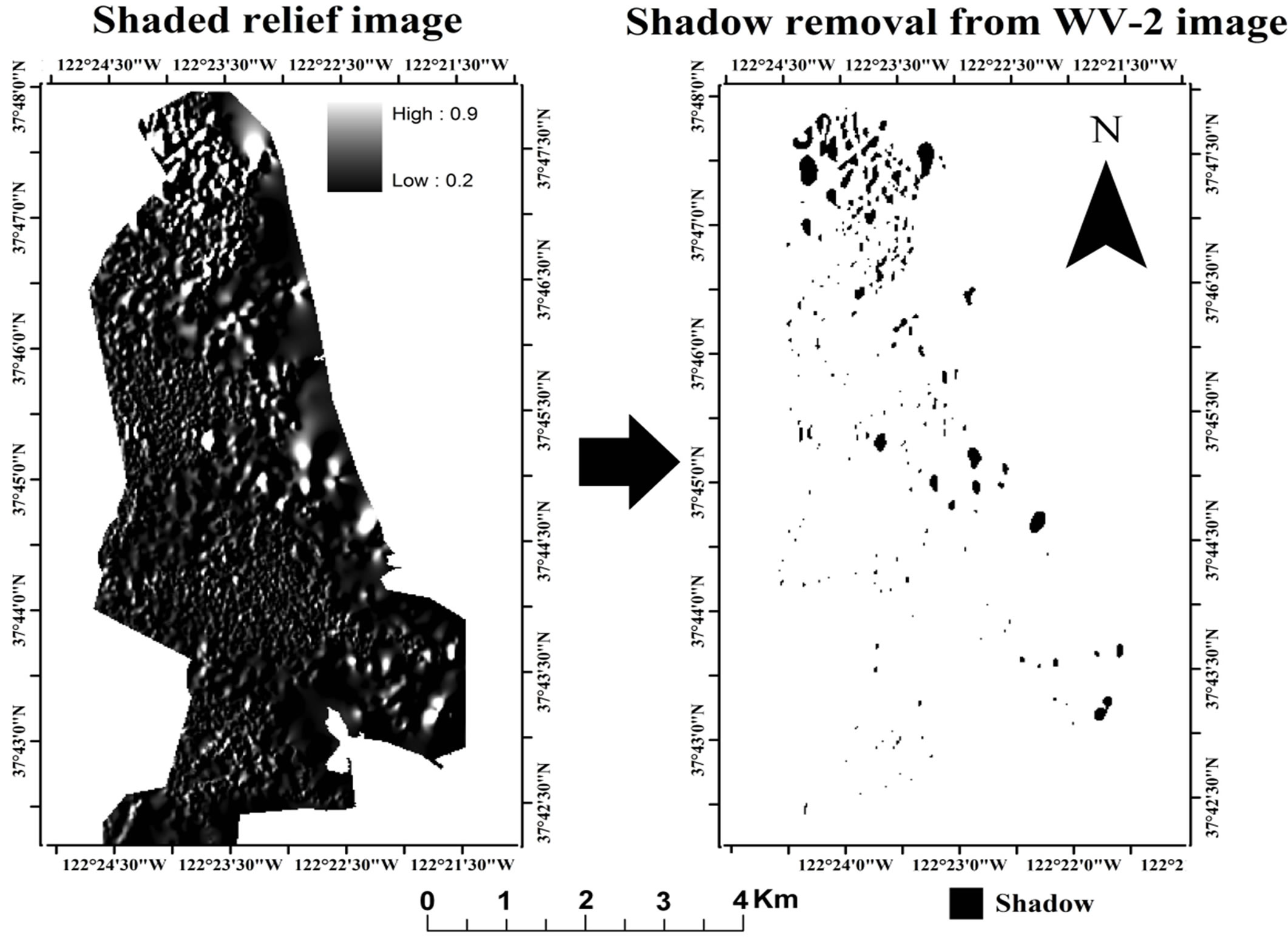
Figure 5. DSM-based shaded relief map and shadow map for the study area.
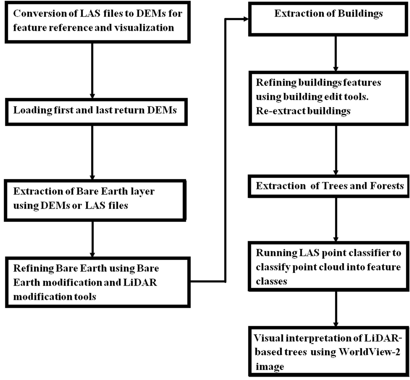
Figure 6. LiDAR point cloud data processing workflow adapted in the present study.
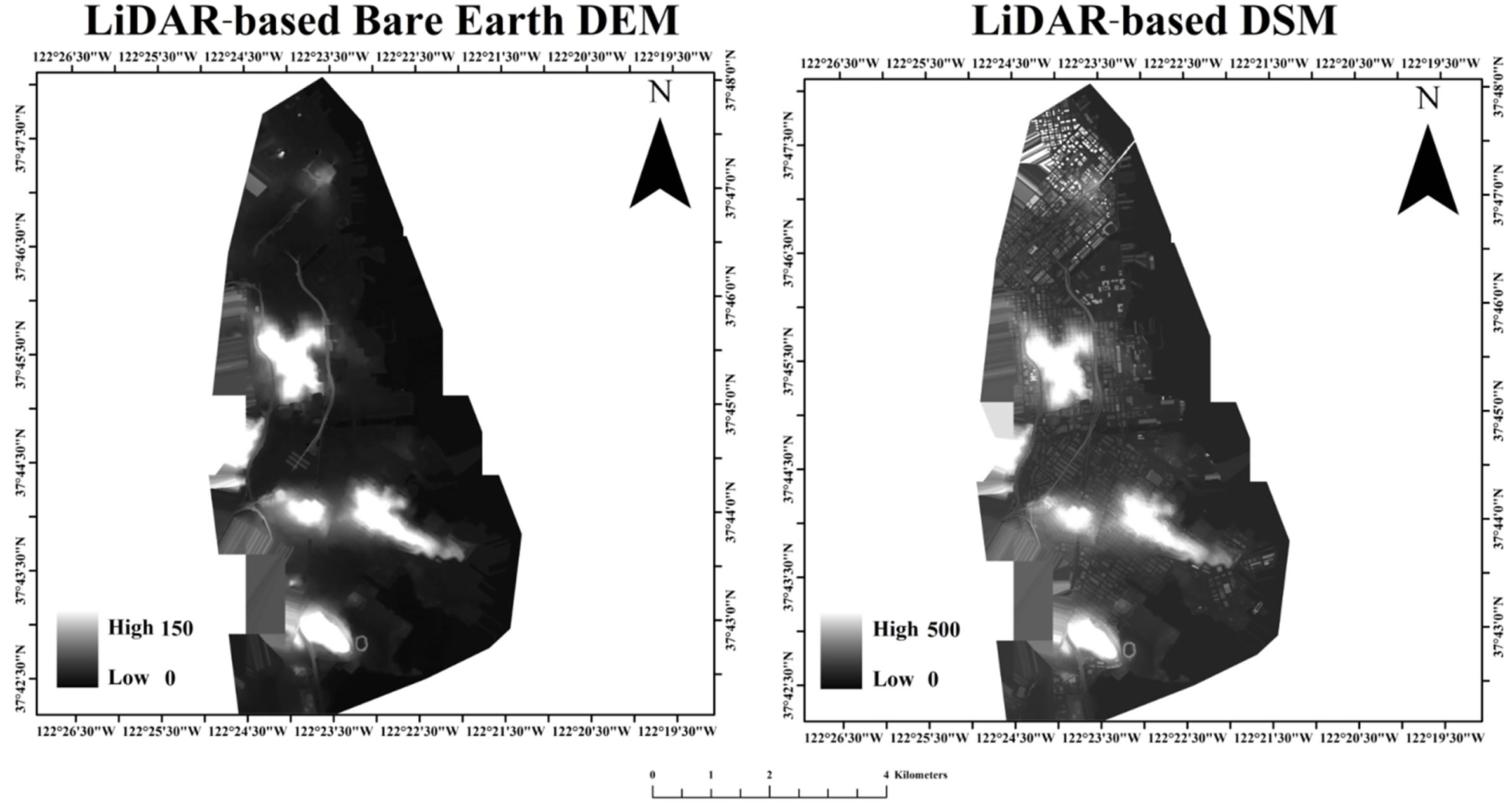
Figure 7. LiDAR based bare earth DEM and DSM for the study area.
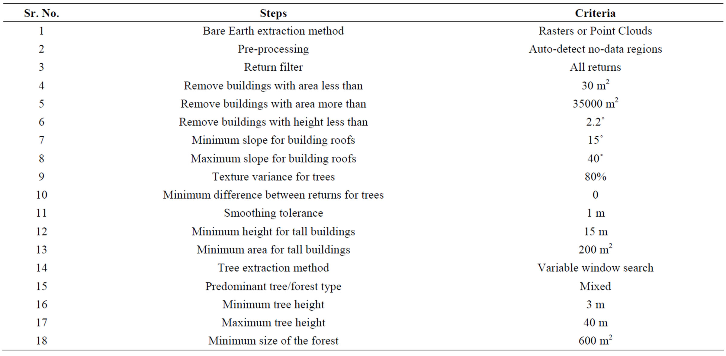
Table 1. Criteria used for bare earth, buildings and trees extraction.
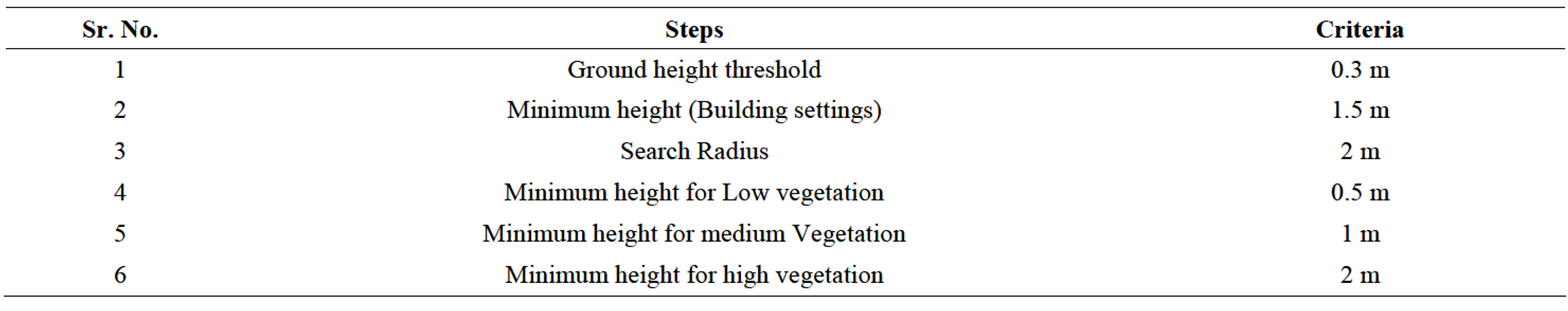
Table 2. Criteria for point cloud classification.
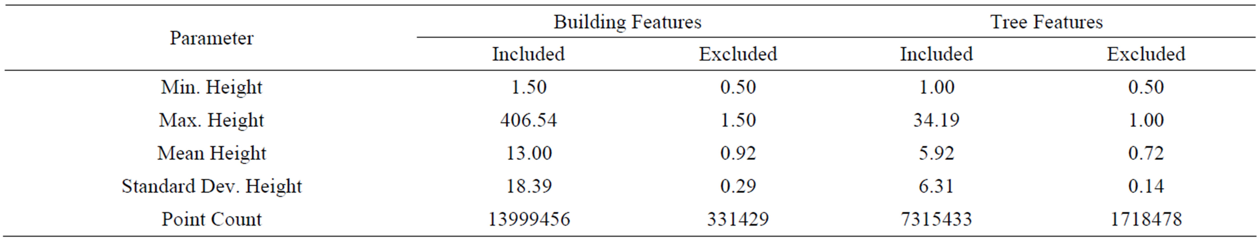
Table 3. LAS classification statistics for building and tree class (height statistics for LAS points which were classified as a given feature class are recorded in the “Included” field, and statistics in the “Excluded” field were gathered from points that should have been classified as the given feature class but were weeded out due to the user-defined classification settings).
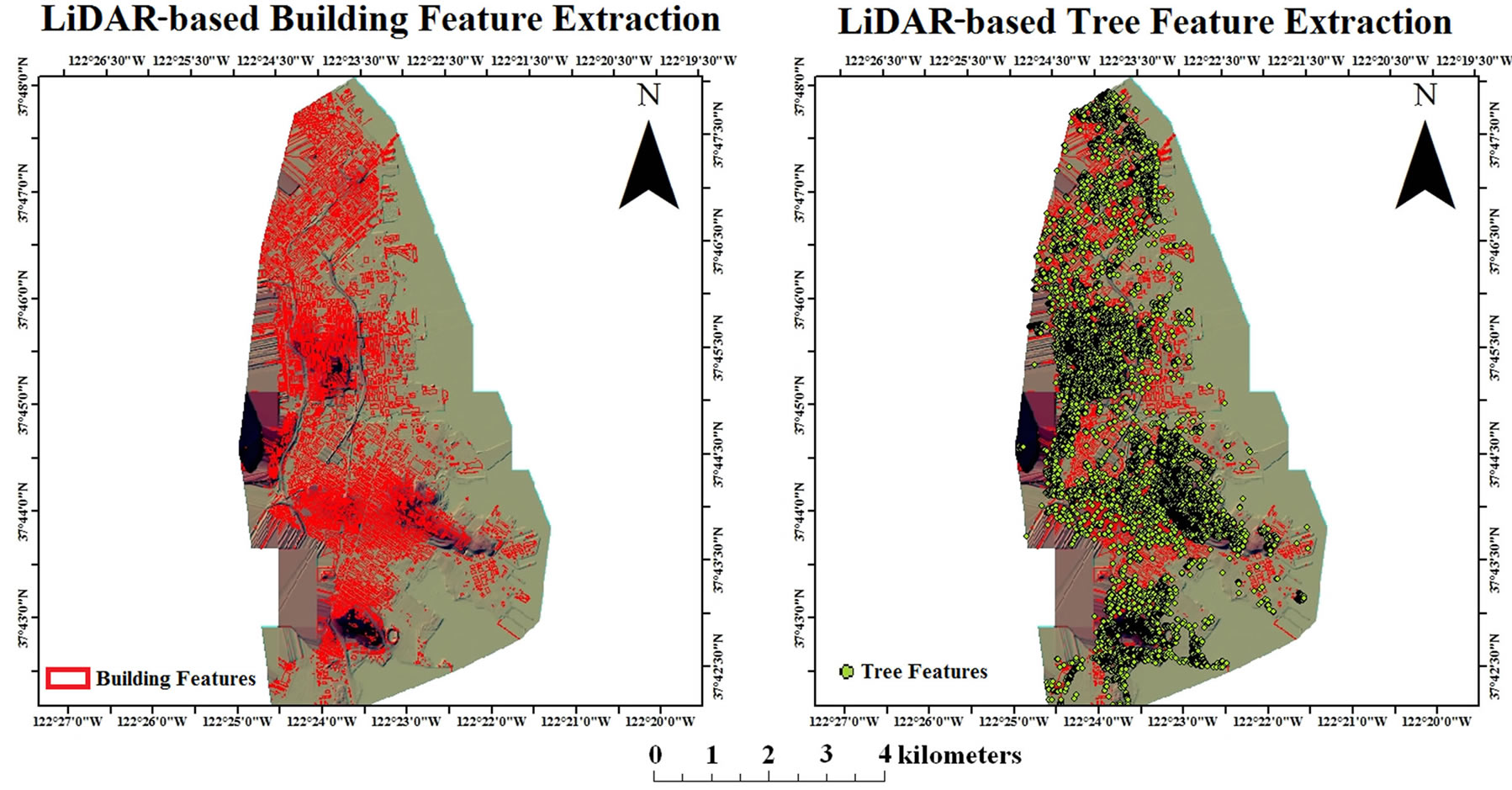
Figure 8. LiDAR-based building and tree features.
extracting the trees, the minimum tree height was set to a value = 0.5 m, that corresponds with the size of vegetation we desire to be called a tree. The resulting shapefile of tree feature extraction consists of point features showing individual trees. While extracting forests, maximum distance between the trees and minimum size of group of the trees/ minimum size of a forest were specified by trial and error method to achieve desired results. After tree feature extraction, LiDAR point cloud classification was performed so as to classify different points according to their elevation values and defined criteria. The accuracy of the classification highly depends on the user defined criteria (Table 1 and 2). Texture variance for trees and minimum difference between returns for trees are the crucial parameters which affect the extraction accuracy. The classified LiDAR output contained three categories: bare earth, buildings and vegetation. The text file of output gives information about the total points included or excluded in a particular class, maximum height, minimum height, etc. (Table 3). The segmented point clouds and the tree locations are then used as input for tree filtering routine.
3.2.4. Tree Filtering
Since the data includes many elevated objects such as buildings, trees and bridges, the classification or filtering is needed in various LiDAR applications. The classification of point cloud data is called the filtering process of LiDAR data. In this study, a tree filtering algorithm aims at separating dominant trees and above-ground objects such as buildings, bridges and undergrowth vegetation. This algorithm requires three input parameters: 1) maximum growing distance for tree crown, 2) maximum growing distance for tree trunk, and 3) average tree trunk diameter. We used the histogram-based tree filtering algorithm practiced by Rahman et al. [35]. The final output map of tree feature extraction is shown in Figure 8 and 3-D rendering is shown in Figure 9.
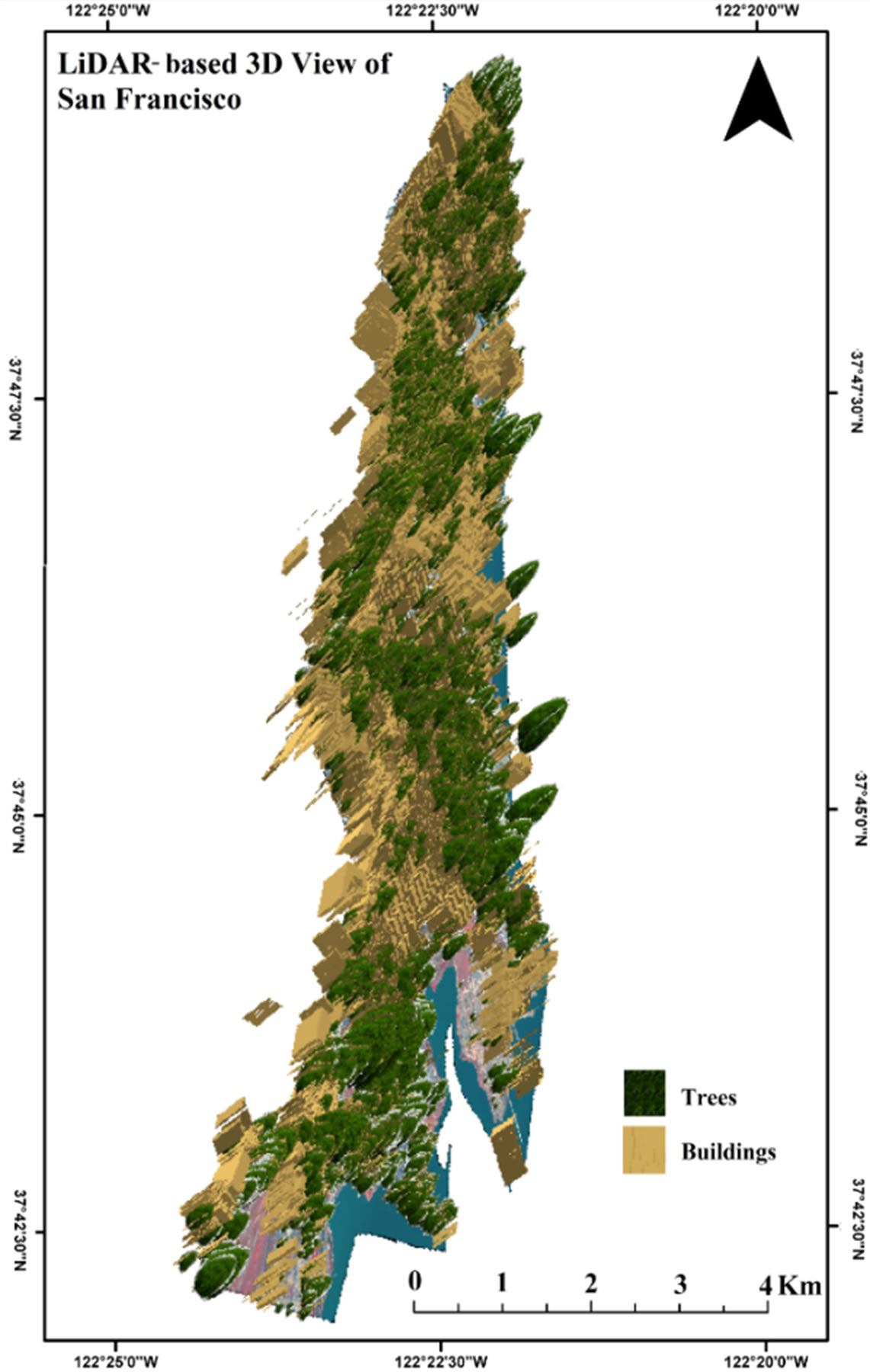
Figure 9. 3D rendering of extracted tree and building features over the study area extraction results.
3.2.5. Accuracy Assessment
In accuracy assessment, we visually interpreted the LiDAR-classified trees on WorldView-2 image. The 8- band WorldView-2 image was georeferenced, orthorectified and PAN-sharpened using HCS method (Figure 10). WV-2 PAN-sharpened image (0.5 m) was used such that the tree features can be easily recognized. The PANsharpened image (0.5 m) was visualized in ArcGIS 10 at several scales for the better visualization of tree features using various band combinations: 7-4-2; 8-7-2; 6-3-2; 5-3-2 and 7-3-2. Finally, 1:500 scale and 5-3-2 band combination was selected for visualization of the tree features. Based on publically available map datasets and Google images of the study area and visual analysis of the satellite data, the WV-2 HCS-sharpened image was manually evaluated using ArcGIS 10 to visualize against LiDAR based extracted tree features. All the tree features extracted by processing LiDAR data were evaluated using WW-2 PAN-sharpened image to interpret individual trees for statistical accuracy assessment.
4. Results
Our research focused on CHM-based tree feature extraction using high-resolution airborne LiDAR data and its accuracy assessment using high-resolution WV-2 image data. In tree feature extraction methodology, the scene dependent criteria were used. Texture variance for tree features and minimum difference between returns for trees were the crucial parameters in building and trees feature extraction. The results depicted on Table 3 show that all the LiDAR points exihibit point cloud classification and hence, the criteria used for tree and building feature extraction were appropriate. A 3D representation of the extracted tree features is depicted in Figure 11.
A 8-band WV-2 image was used for visual interpretation of LiDAR-classified tree features. The image was PAN-sharpened and georeferenced which helped in proper visualization of LiDAR tree points. In addition, orthorectification of WV-2 images enhanced the overall accuracy of the analysis.
The results depicted on Table 4 show that 15,143 tree features were extracted by CHM method using LiDAR point cloud data. All the tree features extracted using LiDAR data were cross-verified using multitemporal high resolution image, which indicates that the 14,841 tree features were correctely interepreted out of 15,143 tree features. The overall accuracy of LiDAR based tree feature extraction was found to be 98% against the high resolution satellite image as a reference.
A DSM-based shadow mask was used for reducing the potential source of error attributable to topography-based shadow in high resolution image. A total of 1011 tree features under shadow were cross-verified using multitemporal image data. It is evident that the LiDAR-based extraction caused over-estimation of 302 tree features, which can be atttributed to two methodological and experimental inadequacies: 1) the present research was carried out using scene dependent criteria which should be optimized with trial-and-error method, and 2) the error might be propogated during the LiDAR filtering or classification process. For optimal tree feature extraction, we propose the rigorous optimization of criteria and synergetic usage of high resolution data for tree feature extraction in future studies.
5. Discussion
Separation of point cloud into ground and non-ground is the most critical step for DEM/DTM generation from point cloud data. Filtering and interpolation algorithms play a major role in this task. As point cloud is able to penetrate the forested areas, it has an advantage over photogrammetry of a highly accurate DTM extraction in forested areas [10]. Numerous methods have been developed for point cloud processing so far, but some more
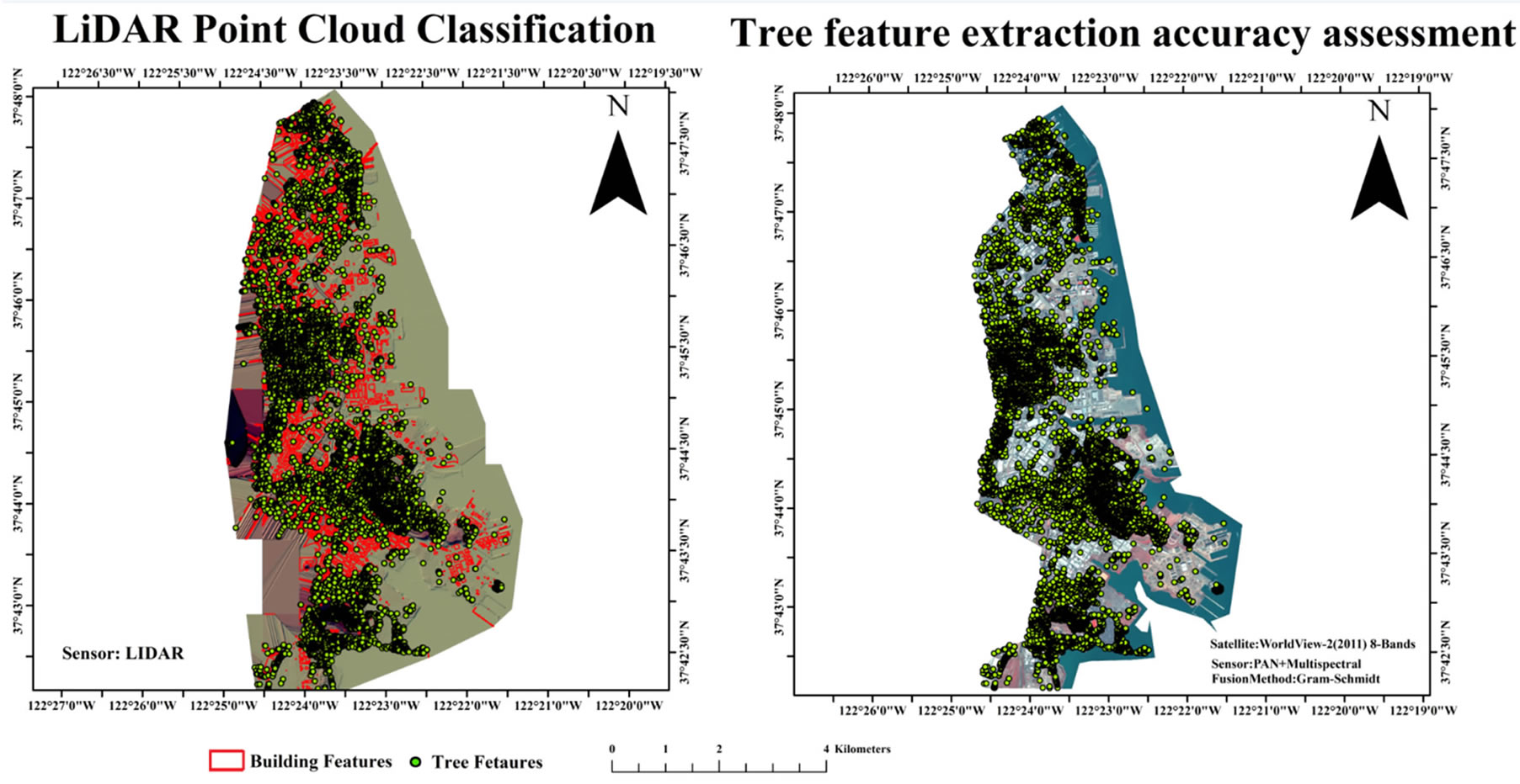
Figure 10. LiDAR-based classification and tree feature extraction accuracy assessment.
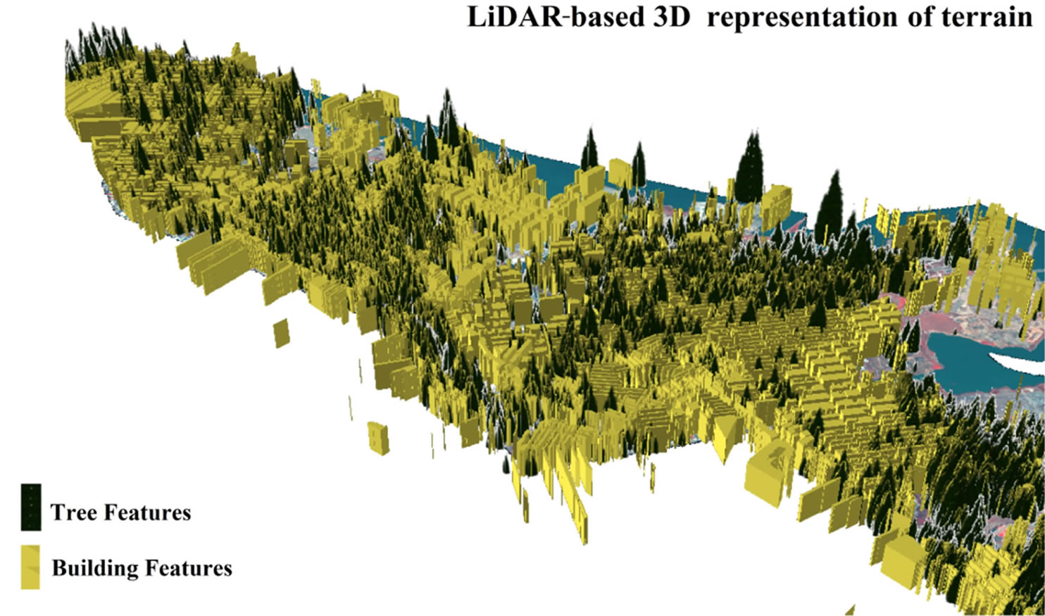
Figure 11. 3D representation of extracted tree features over the study area.
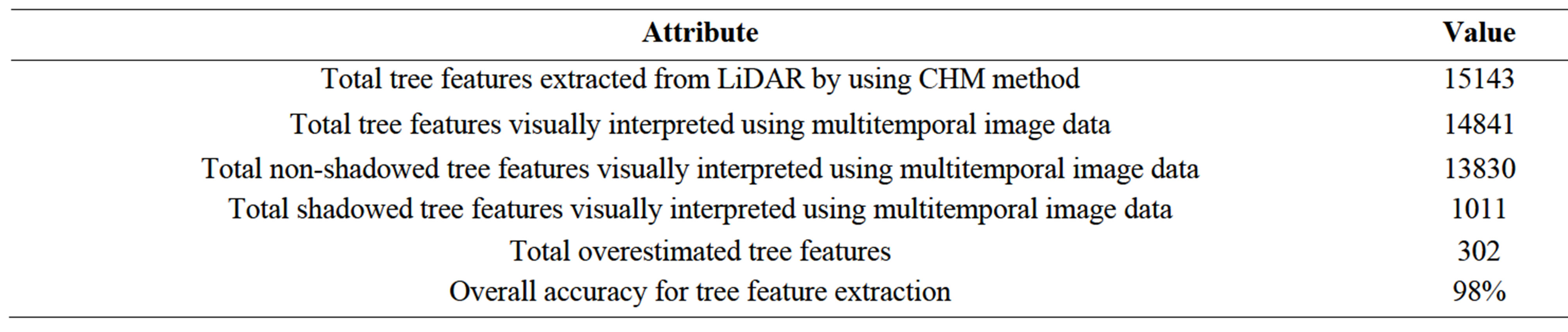
Table 4. Statistics for LiDAR based tree feature extraction.
work has to be done to get much better results. High density datasets make it easy to filter ground from nonground points, but for low density datasets, choice of filtering algorithm is an utmost important step to achieve the highest possible accuracy. Due to significant increase in the volume in case of highly dense point cloud data, data storage, processing and manipulation become important issues to be taken care of [63]. We note that the use of a PAN-sharpened image as reference data for the accuracy analysis introduces, to some extent, data circularity. We cross-verified the tree features visually interpreted on PAN-sharpened WV-2 images with multitemporal satellite image data to reduce data circularity and bias due to visual interpretation of WV-2 data. Additionally, we have carried out an extensive accuracy analysis of the tree feature extraction using the visual interpretation of WV-2 image supported by empirical crossverification of tree points in terms of visual analysis of Google Earth images of the study area and employing different methods using various sources of ground truth data acquired through several means from urban areas, which are publicly available (GIS-based) as maps and manually prepared polygons. We also note that the difference in acquisition of WV-2 and LiDAR datasets might have affected the analysis, however, this study employs many supplementary temporal datasets in the analysis. Therefore, we surmise that the potential data circularity existing in our accuracy analysis had a relatively insignificant effect on the comparative performance of the tree feature extraction.
6. Conclusion
The high resolution airborne LiDAR data provide tremendous potential for tree feature extraction in urban environment and the high resolution WV-2 imagery supplements the accuracy assessment procedure. The objective of this study was to evaluate CHM-based tree-feature extracting accuracy by visual interpretation/identification on 8-band WorldView-2 image. Our study uses the algorithm developed by Overwatch system’s LiDAR Analyst for ArcGIS for LiDAR feature extraction and classification with scene dependent criteria. The 8-band WorldView-2 image gives better recognition and extraction of various land-cover features and due to the inclusion of new bands in that image, the vegetation analysis becomes more effective. This study leads to the following conclusions: 1) Texture variance for trees and minimum difference between returns for trees turned out to be the two most important factors in discriminating the tree and building features in the LiDAR data; 2) Preprocessing of the WV-2 image improved the visualization of vegetation features; 3) LiDAR data were found to be capable of extracting shadow-covered tree features; 4) LiDAR point cloud data can be used in conjunction with satellite image data for supporting tree feature extraction. The research highlights the usefulness of the commonly used methodology for the LiDAR data processing and the effectiveness of 8-band WorldView-2 remotely sensed imagery for accuracy assessment of LiDAR-based tree-feature extraction capability.
7. Acknowledgements
We are indebted to the organizers of the IEEE GRSS Data Fusion Contest (2012), who provided the research platform and images to our research team free of cost. We also acknowledge Dr. Rajan, Director, NCAOR and Mr. R. Ravindra, ex-Director, for their encouragement and motivation for this research. This is NCAOR contribution No. 17/2013.
REFERENCES
- M. A. Lefsky, W. B. Cohen, G. G. Parker and D. J. Harding, “Lidar Remote Sensing for Ecosystem Studies,” BioScience, Vol. 52, No. 1, 2002, pp. 19-23. http://dx.doi.org/10.1641/0006-3568(2002)052[0019:LRSFES]2.0.CO;2
- A. Wehr and U. Lohr, “Airborne Laser Scanning—An Introduction and Overview,” ISPRS Journal of Photogrammetry and Remote Sensing, Vol. 54, No. 2-3, 1999, pp. 68-82. http://dx.doi.org/10.1016/S0924-2716(99)00011-8
- D. L. A. Gaveau and R. A. Hill, “Quantifying Canopy Height Underestimation by Laser Pulse Penetration in Small-Footprint Airborne Laser Scanning Data,” Canadian Journal of Remote Sensing, Vol. 29, No. 5, 2003, pp. 650-657. http://dx.doi.org/10.5589/m03-023
- C. Hopkinson, L. Chasmer, C. Young-Pow and P. Treitz, “Assessing Forest Metrics with a Ground-Based Scanning Lidar,” Canadian Journal of Forest Research, Vol. 34, No. 3, 2004, pp. 573-583. http://dx.doi.org/10.1139/x03-225
- C. Hopkinson, M. Sitar, L. Chasmer and P. Treitz, “Mapping Snowpack Depth Beneath Forest Canopies Using Airborne Lidar,” Photogrammetric Engineering & Remote Sensing, Vol. 70, No. 3, 2004, pp. 323-330.
- N. F. Glenn, D. R. Streutker, D. J. Chadwick, G. D. Thackray and S. J. Dorsch, “Analysis of LiDAR-Derived Topographic Information for Characterizing and Differentiating Landslide Morphology and Activity,” Geomorphology, Vol. 73, No. 1-2, 2006, pp. 131-148. http://dx.doi.org/10.1016/j.geomorph.2005.07.006
- S.-J. Lee, Y.-C. Chan, D. Komatitsch, B.-S. Huang and J. Tromp, “Effects of Realistic Surface Topography on Seismic Ground Motion in the Yangminshan Region of Taiwan Based upon the Spectral-Element Method and LiDAR DTM,” Bulletin of the Seismological Society of America, Vol. 99, No. 2A, 2009, pp. 681-693. http://dx.doi.org/10.1785/0120080264
- T. Brandtberg, T. A. Warner, R. E. Landenberger and J. B. McGraw, “Detection and Analysis of Individual Leaf-Off Tree Crowns in Small Footprint, High Sampling Density Lidar Data from the Eastern Deciduous Forest in North America,” Remote Sensing of Environment, Vol. 85, No. 3, 2003, pp. 290-303. http://dx.doi.org/10.1016/S0034-4257(03)00008-7
- National Oceanic and Atmospheric Administration (NOAA) Coastal Services Center, “Lidar 101: An Introduction to Lidar Technology, Data, and Applications,” NOAA Coastal Services Center, Charleston, 2012.
- X. Liu, “Airborne Point Cloud for DEM Generation: Some Critical Issues,” Progress in Physical Geography, Vol. 32, No. 1, 2008, pp. 31-49. http://dx.doi.org/10.1177/0309133308089496
- E. S. Anderson, J. A. Thompson and R. E. Austin, “LiDAR Density and Linear Interpolator Effects on Elevation Estimates,” International Journal of Remote Sensing, Vol. 26, No. 18, 2005, pp. 3889-3900. http://dx.doi.org/10.1080/01431160500181671
- C. Childs, “Interpolation Surfaces in ArcGIS Spatial Analyst,” ArcUser, July-September 2004, pp. 32-35.
- T. Podobnikar, “Suitable DEM for Required Application,” Proceedings of the 4th International Symposium on Digital Earth, Tokyo, March 2005.
- N. A. Cressie, “Statistics for Spatial Data,” Wiley, New York, 1993.
- P. J. J. Desmet, “Effects of Interpolation Errors on the Analysis of DEMs,” Earth Surface Processes and Landforms, Vol. 22, No. 6, 1997, pp. 563-580. http://dx.doi.org/10.1002/(SICI)1096-9837(199706)22:6<563::AID-ESP713>3.0.CO;2-3
- Q. Chen, D. Baldocchi, P. Gong and M. Kelly, “Isolating Individual Trees in a Savanna Woodland Using Small Footprint Lidar Data,” Photogrammetric Engineering & Remote Sensing, Vol. 72, No. 8, 2006, pp. 923-932.
- Q. Chen, P. Gong, D. Baldocchi and Y. Q. Tian, “Estimating Basal Area and Stem Volume for Individual Trees from Lidar Data,” Photogrammetric Engineering & Remote Sensing, Vol. 73, No. 12, 2007, pp. 1355-1365.
- B. Koch, U. Heyder and H. Weinacker, “Detection of Individual Tree Crowns in Airborne Lidar Data,” Photogrammetric Engineering & Remote Sensing, Vol. 72, No. 4, 2006, pp. 357-363.
- I. Korpela, B. Dahlin, H. Schäfer, E. Bruun, F. Haapaniemi, J. Honkasalo, S. Ilvesniemi, V. Kuutti, M. Linkosalmi, J. Mustonen, M. Salo, O. Suomi and H. Virtanen, “Single-Tree Forest Inventory Using Lidar and Aerial Images for 3D Treetop Positioning, Species Recognition, Height and Crown Width Estimation,” International Archives of Photogrammetry, Remote Sensing and Spatial Information Sciences (IAPRS), Vol. 36, Pt. 3, 2007, pp. 227-233.
- X. Yu, J. Hyyppä, M. Vastaranta, M. Holopainen and R. Viitala, “Predicting Individual Tree Attributes from Airborne Laser Point Clouds Based on the Random Forests Technique,” ISPRS Journal of Photogrammetry and Remote Sensing, Vol. 66, No. 1, 2011, pp. 28-37. http://dx.doi.org/10.1016/j.isprsjprs.2010.08.003
- S. Lang, D. Tiede, B. Maier and T. Blaschke, “3D Forest Structure Analysis from Optical and LIDAR Data,” Revista Ambiência, Guarapuava, v.2 Edição Especial, Vol. 1, No. 1, 2006, pp. 95-110.
- S. C. Popescu, R. H. Wynne and R. F. Nelson, “Estimating Plot Level Tree Heights with Lidar: Local Filtering with a Canopy Height Based Variable Window Size,” Computers and Electronics in Agriculture, Vol. 37, No. 1-3, 2002, pp. 71-95. http://dx.doi.org/10.1016/S0168-1699(02)00121-7
- K. Lim, P. Treitz, M. Wulder, B. St-Ongec and M. Flood, “LiDAR Remote Sensing of Forest Structure,” Progress in Physical Geography, Vol. 27, No. 1, 2003, pp. 88-106. http://dx.doi.org/10.1191/0309133303pp360ra
- S. C. Popescu, R. H. Wynne and R. F. Nelson, “Measuring Individual Tree Crown Diameter with Lidar and Assessing Its Influence on Estimating Forest Volume and Biomass,” Canadian Journal of Remote Sensing, Vol. 29, No. 5, 2003, pp. 564-577. http://dx.doi.org/10.5589/m03-027
- G. Patenaude, R. A. Hill, R. Milne, D. L. A. Gaveau, B. B. J. Briggs and T. P. Dawson, “Quantifying Forest above Ground Carbon Content Using LiDAR Remote Sensing,” Remote Sensing of Environment, Vol. 93, No. 3, 2004, pp. 368-380. http://dx.doi.org/10.1016/j.rse.2004.07.016
- S. C. Popescu and R. H. Wynne, “Seeing the Trees in the Forest: Using Lidar and Multispectral Data Fusion with Local Filtering and Variable Window Size for Estimating Tree Height,” Photogrammetric Engineering & Remote Sensing, Vol. 70, No. 5, 2004, pp. 589-604.
- D. Riaño, E. Chuvieco, S. Condés, J. González-Matesanz and S. L. Ustin, “Generation of Crown Bulk Density for Pinus sylvestrisL. from Lidar,” Remote Sensing of Environment, Vol. 92, No. 3, 2004, pp. 345-352. http://dx.doi.org/10.1016/j.rse.2003.12.014
- J. C. Suárez, C. Ontiveros, S. Smith and S. Snape, “Use of Airborne LiDAR and Aerial Photography in the Estimation of Individual Tree Heights in Forestry,” Computers & Geosciences, Vol. 31, No. 2, 2005, pp. 253-262. http://dx.doi.org/10.1016/j.cageo.2004.09.015
- S. C. Popescu, “Estimating Biomass of Individual Pine Trees Using Airborne Lidar,” Biomass and Bioenergy, Vol. 31, No. 9, 2007, pp. 646-655. http://dx.doi.org/10.1016/j.biombioe.2007.06.022
- S. D. Roberts, et al., “Estimating Individual Tree Leaf Area in Loblolly Pine Plantations Using LiDAR-Derived Measurements of Height and Crown Dimensions,” Forest Ecology and Management, Vol. 213, No. 1-3, 2005, pp. 54-70. http://dx.doi.org/10.1016/j.foreco.2005.03.025
- M. Heurich, “Automatic Recognition and Measurement of Single Trees Based on Data from Airborne Laser Scanning over the Richly Structured Natural Forests of the Bavarian Forest National Park,” Forest Ecology and Management, Vol. 255, No. 7, 2008, pp. 2416-2433. http://dx.doi.org/10.1016/j.foreco.2008.01.022
- D. A. Zimble, D. L. Evans, G. C. Calrson and R. C. Parker, “Characterizing Vertical Forest Structure Using Small-Footprint Airborne LiDAR,” Remote Sensing of Environment, Vol. 87, No. 2-3, 2003, pp. 171-182. http://dx.doi.org/10.1016/S0034-4257(03)00139-1
- M. Z. A. Rahman and B. Gorte, “Tree Filtering for High Density Airborne LiDAR Data,” In: R. Hill, J. Rosette and J. Suarez (Eds.), Proceedings of the Silvilaser 2008: 8th International Conference on LiDAR Applications in Forest Assessment and Inventory, Heriot-Watt University, Edinburgh, 2008, pp. 544-553.
- M. Z. A. Rahman and B. G. H. Gorte, “Tree Crown Delineation from High-Resolution Airborne LiDAR Based on Densities of High Points,” Proceedings of ISPRS Workshop Laserscanning 2009, Paris, 1-2 September 2009, pp. 123-128. http://www.isprs.org/proceedings/XXXVIII/3-W8/papers/p51.pdf
- M. Z. A. Rahman and B. G. H. Gorte, “A New Method for Individual Tree Delineation and Undergrowth Removal from High Resolution Airborne LiDAR,” Proceedings of ISPRS Workshop Laserscanning 2009, Paris, 1-2 September 2009, pp. 283-288. http://www.isprs.org/proceedings/XXXVIII/3-W8/papers/p52.pdf
- J. Reitberger, M. Heurich, P. Krzystek and U. Stilla, “Single Tree Detection in Forest Areas with High-Density LiDAR Data,” International Archives of Photogrammetry, Remote Sensing and Spatial Information Sciences, Vol. 36, No. 3, 2007, pp. 139-144.
- D. Tiede, G. Hochleitner and T. Blaschke, “A Full GISBased Workflow for Tree Identification and Tree Crown Delineation Using Laser Scanning,” In: U. Stilla, F. Rottensteiner and S. Hinz, Eds., Proceedings of CMRT 05, International Archives of Photogrammetry and Remote Sensing, XXXVI(Part 3/W24), Vienna, 29-30 August 2005, pp.9-14.
- M. J. Falkowski, A. M. S. Smith, A. T. Hudak, P. E. Gessler, L. A. Vierling and N. L. Crookston, “Automated Estimation of Individual Conifer Tree Height and Crown Diameter via Two-Dimensional Spatial Wavelet Analysis of Lidar Data,” Canadian Journal of Remote Sensing, Vol. 32, No. 2, 2006, pp. 153-161. http://dx.doi.org/10.5589/m06-005
- Q. Guo, M. Kelly, P. Gong and D. Liu, “An Object-Based Classification Approach in Mapping Tree Mortality Using High Spatial Resolution Imagery,” GIScience & Remote Sensing, Vol. 44, No. 1, 2007, pp. 24-47. http://dx.doi.org/10.2747/1548-1603.44.1.24
- F. Morsdorf, E. Meier, B. Kötz, K. I. Itten, M. Dobbertin and B. Allgowe, “LIDAR-Based Geometric Reconstruction of Boreal Type Forest Stands at Single Tree Level for Forest and Wildland Fire Management,” Remote Sensing of Environment, Vol. 92, No. 3, 2004, pp. 353-362. http://dx.doi.org/10.1016/j.rse.2004.05.013
- H. Lee, K. C. Slatton, B. E. Roth and W. P. Cropper Jr., “Adaptive Clustering of Airborne LiDAR Data to Segment Individual Tree Crowns in Managed Pine Forests,” International Journal of Remote Sensing, Vol. 31, No. 1, 2010, pp. 117-139. http://dx.doi.org/10.1080/01431160902882561
- D. J. Nowak, R. E. Hoehn III, D. E. Crane, J. C. Stevens and J. T. Walton, “Assessing Urban Forest Effects and values, San Francisco’s Urban Forest,” Resource Bulletin NRS-8., U.S. Department of Agriculture, Forest Service, Northern Research Station, Newtown Square, 2007, p. 22
- P. Teillet, M. Fedosejevs, D. Gauthier, M. A. D’Iorio, B. Rivard and P. Budkewitsch, “Initial Examination of Radar Imagery of Optical Radiometric Calibration Sites,” SPIE Proceedings, Vol. 2583, 1995, pp. 154-165. http://dx.doi.org/10.1117/12.228560
- P. S. Chavez, “Image-Based Atmospheric CorrectionsRevisited and Improved,” Photogrammetric Engineering and Remote Sensing, Vol. 62, No. 9, 1996, pp.1025-1036.
- C. Song, C. E. Woodcock, K. C. Seto, M. P. Lenney and S. A. Macomber, “Classification and Change Detection Using Landsat TM Data: When and How to Correct Atmospheric Effects,” Remote Sensing of Environment, Vol. 75, No. 2, 2001, pp. 230-244. http://dx.doi.org/10.1016/S0034-4257(00)00169-3
- S. D. Jawak and A. J. Luis, “Improved Land Cover Mapping Using High Resolution Multiangle 8-Band WorldView-2 Satellite Remote Sensing Data,” Journal of Applied Remote Sensing, Vol. 7, No. 1, 2013, Article ID: 073573. http://dx.doi.org/10.1117/1.JRS.7.073573
- H. W. Bakker, W. F. Feringa, et al., “Principles of Remote Sensing,” The International Institute for GeoInformation Science and Earth Observation (ITC), Enschede, 2009.
- T. Updike and C. Comp, “Radiometric Use of Worldview-2 Imagery,” Technical Note, Digitalglobe®, Colorado [online], 2013. www.digitalglobe.com/downloads/Radiometric_Use_of_WorldView-2_Imagery.pdf
- S. D. Jawak and A. J. Luis, “A Comprehensive Evaluation of PAN-Sharpening Algorithms Coupled with Resampling Methods for Image Synthesis of very High Resolution Remotely Sensed Satellite Data,” Advances in Remote Sensing, Vol. 2, No. 4, 2013, Article ID: 2630049.
- S. D. Jawak and A. J. Luis, “Applications of Worldview- 2 Satellite Data for Extraction of Polar Spatial Information and DEM of Larsemann Hills, East Antarctica,” FSNC 2011, Vol. 3, No. 1, 2011, pp. 148-151.
- S. D. Jawak and A. J. Luis, “High Resolution 8-Band WorldView-2 Satellite Remote Sensing Data for Polar Geospatial Information Mining and Thematic Elevation Mapping of Larsemann Hills, East Antarctica,” 11th ISAES- 2011, Edinburgh, 10-16 July 2011.
- S. D. Jawak and J. Mathew, “Semi-Automatic Extraction of Water Bodies and Roads from High Resolution QuickBird Satellite Data,” Proceedings of Geospatial World Forum 2011, Vol. PN-263, No. 1, 18-21 January 2011, pp. 247-257.
- S. D. Jawak, P. S. Khopkar and A. J. Luis, “Spectral Index Ratio-Based Quantitative Analysis of WorldView-2 Pansharpened Data,” National Seminar on Earth Observation & Geo-information Sciences for Environment and Sustainable Development (EGESD), University of Mumbai, Mumbai, 7-9 February 2013.
- S. D. Jawak and A. J. Luis, “WorldView-2 Satellite Remote Sensing Data for Polar Geospatial Information Mining of Larsemann Hills, East Antarctica,” Proceedings of 11th Pacific (Pan) Ocean Remote Sensing Conference (PORSEC), Kochi, 5-9 November 2012, Article ID: PORSEC2012-24-00006.
- S. D. Jawak and A. J. Luis, “Hyperspatial WorldView-2 Satellite Remote Sensing Data for Polar Geospatial Information Mining of Larsemann Hills, East Antarctica,” XXXII SCAR and Open Science Conference (OSC), Portland, 13-25 July 2012.
- S. D. Jawak, P. S. Khopkar and T. M. Godbole, “Spectral Quality Analysis of Pansharpened Worldview-2 Images using Normalized Difference Vegetation/Water (NDVI/ND WI) Index,” India Geospatial Forum, PN-32, Gurgaon, 7-9 February 2012.
- S. D. Jawak and A. J. Luis, “A Spectral Index RatioBased Antarctic Land-Cover Mapping Using Hyperspatial 8-Band WorldView-2 Imagery,” Polar Science, Vol. 7, No. 1, 2013, pp. 18-38. http://dx.doi.org/10.1016/j.polar.2012.12.002
- C. Padwick, M. Deskevich, F. Pacifici and S. Smallwood, “WorldView 2 Pan-Sharpening,” ASPRS 2010, Annual Conference, San Diego, 2010.
- J.-Y. Rau, N.-Y. Chen and L.-C. Chen, “True Orthophoto Generation of Built-Up Areas Using Multi-View Images,” Photogrammetric Engineering & Remote Sensing, Vol. 68, No. 6, 2002, pp. 581-588.
- P. T. Giles, “Remote Sensing and Cast Shadows in Mountainous Terrain,” Photogrammetric Engineering & Remote Sensing, Vol. 67, No. 7, 2001, pp. 833-839.
- P. Gurram, S. Hu and A. Chan, “Uniform Grid Upsampling of 3D Lidar Point Cloud Data,” Proceedings of the SPIE, Vol. 8650, 2013, Article ID: 86500B.
- Q. Guo, W. Li, H. Yu and O. Alvarez, “Effects of Topographic Variability and Lidar Sampling Density on Several DEM Interpolation Methods,” Photogrammetric Engineering & Remote Sensing, Vol. 76, No. 6, 2010, pp. 701-712. http://dx.doi.org/10.14358/PERS.76.6.701
- T. L. Webster and G. Dias, “An Automated GIS Procedure for Comparing GPS and Proximal LIDAR Elevations,” Computers & Geosciences, Vol. 32, No. 6, 2006, pp. 713-726. http://dx.doi.org/10.1016/j.cageo.2005.08.009
NOTES
*Corresponding author.