Advances in Remote Sensing
Vol.2 No.2(2013), Article ID:32666,5 pages DOI:10.4236/ars.2013.22008
Compression of LiDAR Data Using Spatial Clustering and Optimal Plane-Fitting
Department of Civil Engineering, American University of Sharjah, Sharjah, UAE
Email: atarig@aus.edu
Copyright © 2013 Tarig A. Ali. This is an open access article distributed under the Creative Commons Attribution License, which permits unrestricted use, distribution, and reproduction in any medium, provided the original work is properly cited.
Received February 9, 2013; revised March 10, 2013; accepted March 17, 2013
Keywords: LiDAR; Spatial Clustering; Optimal Plane Fitting
ABSTRACT
With the advancement in geospatial data acquisition technology, large sizes of digital data are being collected for our world. These include airand space-borne imagery, LiDAR data, sonar data, terrestrial laser-scanning data, etc. LiDAR sensors generate huge datasets of point of multiple returns. Because of its large size, LiDAR data has costly storage and computational requirements. In this article, a LiDAR compression method based on spatial clustering and optimal filtering is presented. The method consists of classification and spatial clustering of the study area image and creation of the optimal planes in the LiDAR dataset through first-order plane-fitting. First-order plane-fitting is equivalent to the Eigen value problem of the covariance matrix. The Eigen value of the covariance matrix represents the spatial variation along the direction of the corresponding eigenvector. The eigenvector of the minimum Eigen value is the estimated normal vector of the surface formed by the LiDAR point and its neighbors. The ratio of the minimum Eigen value and the sum of the Eigen values approximates the change of local curvature, which determines the deviation of the surface formed by a LiDAR point and its neighbors from the tangential plane formed at that neighborhood. If the minimum Eigen value is close to zero for example, then the surface consisting of the point and its neighbors is a plane. The objective of this ongoing research work is basically to develop a LiDAR compression method that can be used in the future at the data acquisition phase to help remove fake returns and redundant points.
1. Introduction
The large volumes of spatial data and their products made it necessary to research new data compression techniques. Much research has been focused on developing compression methods for aerial and satellite imagery [1,2]. As a result, a number of image compression techniques have been developed for these types of imagery. These compression techniques can be generally categorized in two classes: 1) one that reduces the number of bits and creates a numerically-identical replica of the original image; and 2) one that creates a much compressed replica of the image, but with much degraded quality [3].
LiDAR sensors generate huge datasets of unstructured point clouds of multiple returns, which may be false signals or correspond to natural or manmade features. Because of its large size, LiDAR data has costly storage and computational requirements [4]. To reduce the size of LiDAR data for effective storage and processing, robust compression methods are being researched. Wu and Amaratunga [5] presented wavelet transform-based triangulated networks (WTIN) method for representing large GIS datasets. The WTIN method, which is based on the second generation wavelet theory, can be used to produce multi-resolution representations of the data. Although this method has produced compact multi-resolution representations of LiDAR data with acceptable quality, more efficient quantization schemes are much needed than the simple threshold operation adopted in the method to compress the data [6,7]. Ali and Mehrabian [8] developed a novel computational paradigm for picking sample points to create a triangulated irregular network (TIN) model from LiDAR data of a flat terrain. This method can be used to remove unwanted and redundant points in over-sampled smooth terrain surfaces and small high resolution objects resulting in a compact TIN model.
The method uses the Voronoi diagram to evaluate the local density of the LiDAR points and identify clusters within the data. Then, points in the same proximity with elevations within a threshold are selected. The Voronoi tree concept is then used to delete the selected points and update the Voronoi diagram. The final TIN is then built using a randomized incremental algorithm. The methods described above can help produce a compressed LiDAR dataset. However, none of these methods can be used to remove unwanted and redundant points in the LiDAR data set. The method presented herein can be used to remove unwanted and redundant LiDAR point; producing a much compressed LiDAR dataset through spatial clustering and optimal plane fitting.
2. Methodology
The method adopted in this research consists of (1) classification and spatial clustering and (2) optimal firstorder plane fitting of the LiDAR dataset. The schematic diagram of Figure 1 summarizes the major steps of our compression method.
First-order plane-fitting helps in identifying the type of surface defined by every LiDAR point and its neighbors, and therefore the removal of unwanted, redundant LiDAR points, and fake LiDAR returns becomes possible. The technical approach adopted in this study is explained below:
2.1. Spatial Clustering of the LiDAR Data
The clustering process in this study was performed in two steps: (a) classification of the digital orthoimage of the study area, which was performed using the Bayesian maximum likelihood classification (BMLC), and (b) spatial clustering of the LiDAR dataset. The goal of spatial clustering is to subdivide the data into separate regions
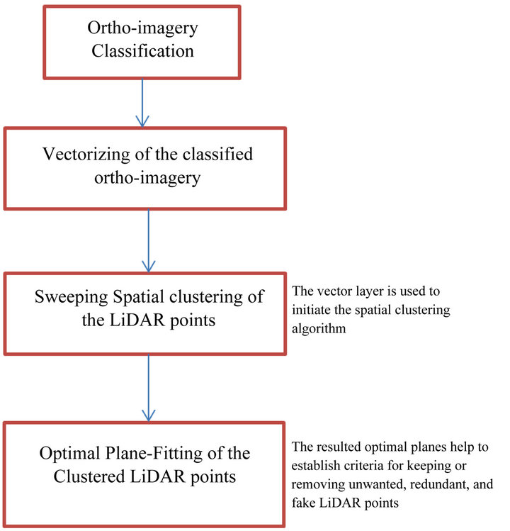
Figure 1. Schematic diagram of the compression method.
that are characterized with a unique property in every region’s local neighborhood. These regions are defined by the points located inside them.
In the BMLC method, a Bayesian Probability Function is calculated based on statistics computed from the inputs for classes established from the training sites. This classification begins with computing statistics for user selected training sites of land cover classes and uses the results of the statistical summary to classify the image. Each pixel is judged as to the class to which it most probably belongs. Histogram analysis was performed to locate image clusters using intensity and distance metric [9]. The 2001 National Land Cover Data (NLCD) Classification Scheme was used when histogram analysis shows the existence of more homogenous regions within the classes resulted from applying the BMLC method. The classified orthoimage of the study area was then vectorized using a run graph method [10]; resulting in a polygon layer. This vectorization method groups pixels in the raster image into area fragments, which were refined using line fitting and line extending processes. Then, the vector layer was used to initiate a sweeping spatial clustering algorithm in order to identify clusters in the LiDAR dataset [11]. Clustering is a well-studied subject and hence many algorithms already exist that can be categorized as hierarchical, partitioning-based, graphbased, density-based algorithms, model-based, and a few combinational algorithms.
The sweeping spatial clustering algorithm was used to determine arbitrary shaped, possibly-nested clusters in the LiDAR dataset. This hierarchical spatial clustering algorithm generates spatial clusters in one pass as it is based on the sweep-line concept which is widely known in computational geometry and computer graphics.
This algorithm works in three phases: initializing, sweeping and finalizing. During the initializing phase, the LiDAR points are sorted according to the direction of the sweep-line movement. In the sweeping phase, a sweep-line moves through the plane and stops to update the data structure when it hits a LiDAR point and it continues until the whole LiDAR point set is clustered. In the finalizing phase, the indices of the resulted clusters are ordered in a simple data structure of arrays.
2.2. Finding Optimal Planes in LiDAR Data
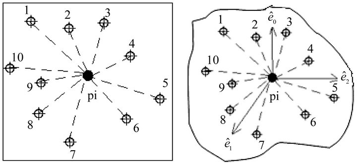
The basic features found in LiDAR point cloud are planes. Having planes, points and edges can be obtained by calculating planes intersections. Two methods are commonly used to identify optimal planes, which are the least square fitting and principal component analysis. First order plane fitting is basically equivalent to the Eigen value problem of the covariance matrix [12], which is the main concept of the principal component analysis method used in this study. Let us first define the point pi and its local neighboring points in the LiDAR point cloud as shown in Figure 2. The point pi in Figure 2 and its neighbors will be used to estimate the surface normal vector.
The covariance matrix of the point pi and its k neighboring points;  is expressed as:
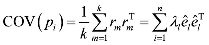
where  is the centroid of pi and its k neighbors, and
 ![]() is the eigenvector of the
is the eigenvector of the  smallest Eigen value
 .
.
Since  is a real, positive, semi-definite matrix, its Eigen values are always greater than or equal to zero. The eigenvector of the minimum Eigen value is the estimated normal vector of the surface formed by pi and its k neighboring points. The other eigenvectors are the tangential vectors of the surface. If the minimum Eigen value is close to zero, then the surface consisting of a LiDAR point and its neighbors is a plane. Note that each Eigen value of the covariance matrix represents the spatial variation along the direction of the corresponding eigenvector. The ratio of the minimum Eigen value and the sum of the Eigen values approximates the change of local curvature, which determines the deviation of the surface formed by a LiDAR point pi and its neighbors from the tangential plane formed at that neighborhood. The optimal planes have been created in this study for the clustered LiDAR points set. And a criterion for keeping or removing unwanted, redundant, and fake LiDAR points has been established based on the optimal plane of the LiDAR dataset obtained using the First Order Plane Fitting method. The success of this compression technique was judged by the compression ratio.
3. Results and Discussion
The LiDAR data used in the work was acquired for a study area in the north east region of the City of Venice, which is located in Sarasota County, Florida, United
 (a) (b)
Figure 2. (a) The LiDAR point pi and its neighbors; (b) The Eigen vectors of covariance matrix of the LiDAR point pi and its k neighbors.
States (Figure 3). The LiDAR dataset for the study area was produced in 2005 for the Southwest Florida Water Management District (SWFWMD) as part of the Manatee/Little Manatee LiDAR Survey project. The data set comprised of 3-D bare earth mass points delivered in the LAS file format based upon the District’s 5000’ × 5000’ grid structure. The LiDAR data (Figure 4) was collected using a Leica LS-50 LiDAR system integrated with an inertial measuring unit (IMU) and a dual frequency GPS receiver. Positional accuracy is 0.75-ft root mean square (RMSE), which satisfies the National Standard for Spatial Data Accuracy (NSSDA) standard for 2-foot contours (scale of 1:12,000). Bare earth LiDAR masspoint data has a vertical accuracy of 0.3-feet root mean square (RMSE). Projected Coordinate System is North American Datum (NAD) of 1983; State Plane System of Florida West and the Vertical datum is the North American Vertical Datum (NAVD) of 1988.
Classification of the study area ortho-imagery was performed using the Bayesian maximum likelihood classification (BMLC) method. The process started by computing statistics for selected training sites of land cover classes and used the results of the statistical summary to
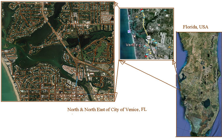
Figure 3. Study area (Intended for color reproduction).

Figure 4. LiDAR data of the study area (Size on disk: 703.32 MB) (Intended for color reproduction).
classify the image. Histogram analysis was performed to locate ortho-image clusters using intensity and distance metrics (Figure 5). The classified ortho-image was sharpened and then a vectorized layer was created using the run graph method resulting in a polygon layer (Figure 6).
The resulted vector layer was then used to initiate a sweeping spatial clustering algorithm in order to identify clusters in the LiDAR dataset following [11]. The algorithm is based on the sweep-line concept which is widely known in computational geometry and computer graphics. The identified clusters in the LiDAR dataset as processed with this algorithm are shown in Figure 7. Optimal planes fitted to the LiDAR dataset (Figure 8) were then generated using the principal component analysis method performed on the clustered LiDAR dataset of Figure 6.
As it can be seen in Figure 7, the sweeping spatial clustering algorithm managed to identify clusters in the LiDAR dataset successfully by separating smooth objects such as buildings tops, pavement, etc. from vegetation and water bodies, even in where these classes are in the same local neighborhood. The spatial clustering of the
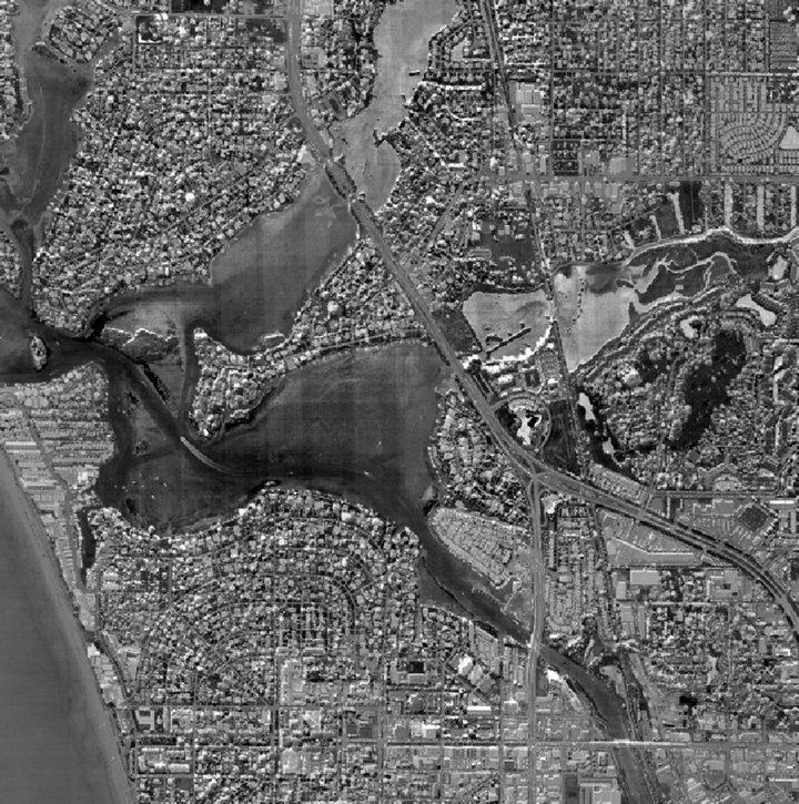
Figure 5. Classified ortho-image of the study area.
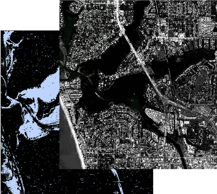
Figure 6. The sharpened calssified orth-image and the vectorized layer of the study area (Intended for color reproduction).
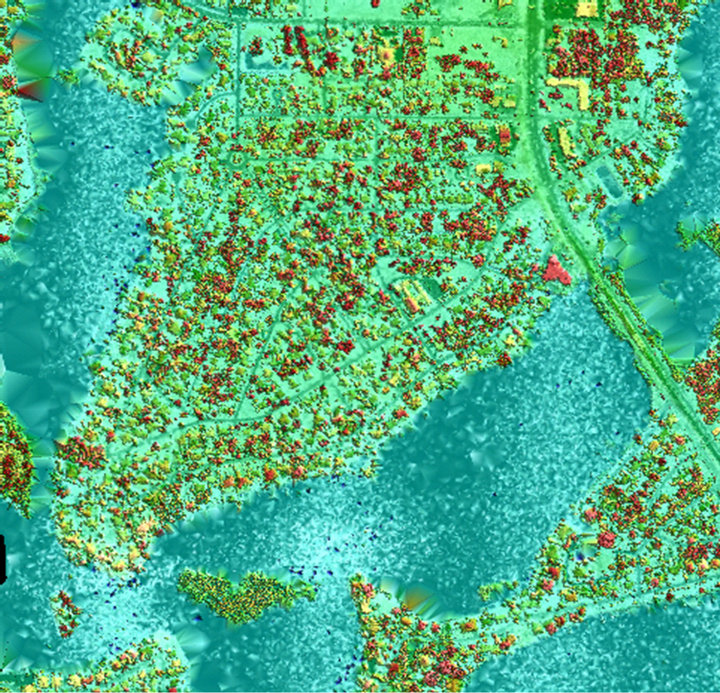
Figure 7. Identified clusters in the LiDAR dataset using the sweeping spatial clustering algorithm (Intended for color reproduction).
 (a)
(a) (b)
(b)
Figure 8. The optimal planes fitted to the LiDAR dataset: (a) 2D View; (b) 3D View (Intended for color reproduction).
LiDAR data in this way helped facilitate the execution of the optimal plane fitting.
Although the optimal planes shown in Figure 8 have been created from the clustered LiDAR dataset shown in Figure 7; we shouldn’t expect the two outcomes to be similar because the optimal plane fitting process by design doesn’t necessary consider the classes in the study area. Optimal plane fitting considers the local neighbored of every LiDAR point regardless of the class to which that point belongs. A keep-or-remove criterion has then been established to remove every LiDAR point that doesn’t fall on one of those optimal planes. All LiDAR points in the study area, which are not located on these optimal planes, have been removed; resulting in a muchcompressed LiDAR dataset that has a smaller size on disk. Specifically, the size of the original LiDAR dataset was 703.32MB and that of the compressed dataset was 578.13MB; resulting in a compression ratio of 17.8%.
4. Conclusion
A LiDAR data compression method was presented in this ongoing research work based on spatial clustering and optimal plane fitting. The method has produced a compression ratio of 17.8% for the LiDAR dataset of the study area, which is promising. The issue this ongoing study is trying to address however is not only the development of a LiDAR compression method with low computational demands. The objective is to develop a compression method that can be applied at the LiDAR acquisition stage that only records the LiDAR points that are on these optimal planes. If this goal is achieved, it will help to design a LiDAR sensor in the future that will only record points that are located on these planes.
REFERENCES
- N. Memon, K. Sayood and S. Magliveras, “Lossless Compression of Multispectral Image Data,” IEEE Transactions on Geoscience and Remote Sensing, Vol. 32, No. 2, 1994, pp. 282-289. doi:10.1109/36.295043
- D. A. Algarni, “Compression of Remotely Sensed Data Using JPEG,” International Archives of Photogrammetry and Remote Sensing, Vol. 31, No. B3, 1996, pp. 24-28.
- Z. Li, X. Yuan and K. Lam, “Effects of JPEG Compression on the Accuracy of Photogrammetric Point Determination,” Journal of Photogrammetric Engineering and Remote Sensing, Vol. 68, No. 8, 2002, pp. 847-853.
- T. A. Ali, “On the Selection of Appropriate Interpolation Method for Creating Coastal Terrain Models from LiDAR Data,” Proceedings of the American Congress on Surveying and Mapping (ACSM) Conference, Nashville, 16- 21 April 2004, 18p.
- J. Wu and K. Amaratunga, “Wavelet Triangulated Irregular Networks,” International Journal of Geographical Information Science, Vol. 17, No. 3, 2003, pp. 273-289. doi:10.1080/1365881022000016016
- B. Pradhan, S. Mansor, A. Ramli, A. Sharif and K. Sandeep, “LIDAR Data Compression Using Wavelets,” Proceedings of Society of Photo-Optical Instrumentation Engineers (SPIE) Conference, Bruges, 19-22 September 2005, pp. 768-786.
- B. Pradhan, S. Kumar, S. Mansor, A. Ramli and A. Sharif, “Light Detection and Ranging (LIDAR) Data Compression,” KMITL Science and Technology Journal, Vol. 5, No. 3, 2005, pp. 515-526.
- T. A. Ali and A. Mehrabian, “A Novel Computational Paradigm for Creating a Triangular Irregular Network (TIN) from LiDAR Data,” Nonlinear Analysis: Theory, Methods and Applications, Vol. 71, No. 12, 2009, pp. 624-629. doi:10.1016/j.na.2008.11.081
- L. Shapiro and G. Stockman, “Computer Vision,” Prentice-Hall, New Jersey, 2001.
- D. Dori and W. Liu, “Sparse Pixel Vectorization: An Algorithm and Its Performance Evaluation,” IEEE Transaction on Pattern Analysis and Machine Intelligence, Vol. 21, No. 3, 1999, pp. 202-215. doi:10.1109/34.754586
- K. Zalik and B. Zalik, “A Sweep-Line Algorithm for Spatial Clustering,” Advances in Engineering Software, Vol. 40, No. 1, 2009, pp. 445-451. doi:10.1016/j.advengsoft.2008.06.003
- K.-H. Bae and D. Lichti, “A Method for Automated Registration of Unorganized Point Clouds,” ISPRS Journal of Photogrammetry & Remote Sensing, Vol. 63, No. 1, 2008, pp. 36-54. doi:10.1016/j.isprsjprs.2007.05.012