American Journal of Plant Sciences
Vol. 4 No. 12B (2013) , Article ID: 40802 , 6 pages DOI:10.4236/ajps.2013.412A2003
Development of Sub-Seasonal Remote Sensing Chlorophyll-A Detection Models
![]()
Brigham Young University, Provo, USA.
Email: carlyahansen@byu.net
Copyright © 2013 Carly Hansen et al. This is an open access article distributed under the Creative Commons Attribution License, which permits unrestricted use, distribution, and reproduction in any medium, provided the original work is properly cited.
Received October 16th, 2013; revised November 18th, 2013; accepted December 1st, 2013
Keywords: Remote Sensing; Chlorophyll Detection; Seasonal Algal Succession
ABSTRACT
Remote sensing techniques are proven methods for quantifying chlorophyll-a levels by inference algal concentrations in reservoirs. One traditional method is to use Landsat imagery and field data from a limited time period to develop a model for a reservoir which relates reflectance in various bands to measured algal (or chlorophyll-a) concentrations and use that model and associated imagery to determine spatial algal concentrations in the reservoir. In this work, we extend these techniques to use historical Landsat data over long time periods to develop seasonal models that will more accurately describe the conditions throughout the growing season. Previous work at Deer Creek included the development of a chlorophyll-a model using data from the months of August to September. This model did not account for seasonal variation and algal succession, which affects the relationship between measured reflectance and algal concentration. Early summer algal blooms are dominated by diatoms (yellow-brown), while the algae vary from chlorophyta (green) in the mid-summer to cyanobacteria (blue-green) in late summer months. This study presents and explores the development and use of seasonal algorithms based on reflective characteristics of various algal communities to create a more accurate model for the reservoir. This study uses water quality data collected over a 20-year period during non-ice conditions along with associated Landsat data. As the field measurements were not taken to support remote sensing measurements, this study evaluates the use of historical data to support remote sensing analysis. It is assumed that reservoir conditions do not change rapidly, the field data can be used to develop correlations with satellite imagery taken within a day of the field measurements, and the seasonal algal communities have different reflective properties (or colors). We present statistical analysis that shows the seasonal algorithms better fit the data than the non-seasonal model and the traditional model calibrated with late-season data. We recommend the use of sub-seasonal algorithms to more accurately model and predict water quality throughout the growing season.
1. Introduction
Deer Creek Reservoir, located in the Rocky Mountain region of the United States, covers approximately 12 square kilometers [1]. The reservoir was formed in 1941 by the creation of an earth-fill dam and today provides water for agricultural and domestic uses for major metropolitan areas in the State of Utah including Salt Lake City. The contributing watershed is approximately 1870 square kilometers, and includes agricultural and livestock grazing, as well as some urban and suburban development. Deer Creek is a popular recreation spot, offering year-round fishing, camping, and water sports.
In the early 1980s, the reservoir was classified as highly eutrophic, with significant algal blooms, high levels of phosphorus, and low dissolved oxygen concentrations. Phosphorus dissolved oxygen and total coliforms exceeded state water quality standards [1]. Problems associated with the large algal blooms ranged from low dissolved oxygen concentrations to reduced recreational use of the reservoir. Ongoing efforts have been made to lower the nutrient loading and to reduce the growth of algal blooms. Initially, these efforts were focused on point pollution sources including municipal wastewater and fish hatchery discharge. Other non-point concerns were nearby dairy operations and erosion. To support these mitigation efforts, a program was implemented to monitor water quality using field sampling methods [1].
Still, as late as 1992, the average Trophic State Index for the reservoir was 45.44, indicating a highly mesotrophic condition, though conditions have improved in subsequent years. Continuing development within the watershed, construction of the upstream Jordanelle reservoir, and on-going mitigation efforts affect nutrient loading and the resultant reservoir conditions. These long-term monitoring data from 1984 to the present, along with significant changes in the watershed, have made Deer Creek Reservoir optimal for study and analysis.
2. Algae Species and Seasonal Succession
In a study from 1991, over 45 unique taxa of algal phytoplankton were identified in Deer Creek [1]. These algae include diatoms, green, and blue-green algae. Monitoring data show that throughout the growing season of AprilSeptember, the reservoir experiences a regular succession of algae growth as the phytoplankton communities dominate during different periods. Studies have shown that in freshwater lakes, diatomic algae peak during the spring, and low production of diatoms occurs during the late summer months [2]. During the low production of diatomic algae, blue-green algae dominate freshwater lakes. Data show that Deer Creek generally follows this cycle.
In temperate regions, such as central Utah, the successive cycle is primarily caused by the minimum and maximums of solar radiation [3], changes in water temperature, sunlight, and nutrient concentration [4]. The relatively high altitude of 5400 ft intensifies these changes. Various phytoplankton communities respond differently to these seasonal conditions, resulting in a definite pattern of succession. In the early months diatoms (yellowbrown in color) dominate, while green algae dominates the mid-summer months, and blue-green algae, including cyanobacteria dominates the reservoir in the later summer months. This effectively divides the growing season into three sub-seasons relating to the type of dominant algae.
Blue-green algae are considered particularly dangerous due to health issues caused by the toxins present in cyanobacteria [4,5]. However, diatoms also have the capacity to negatively affect humans, fish, and the overall ecosystem of a reservoir [6]. For instance, the diatom didymosphenia geminata can cover up to 100 percent of substrate with a thickness of 20 centimeters, significantly impacting the ecosystem and negatively affecting recreational activities. This particular species of diatom has been reported in northern Utah [7] and is a potential threat to lakes in the area, such as Deer Creek Reservoir.
The different populations of algae vary in pigment composition, size and structure, which affect their specific absorption and reflective properties measured by remote sensing techniques [8]. Stuart, Sathyendranath et al. (2000) show that diatoms have lower absorption coefficients compared to other phytoplankton populations and warn that the use of a universal algorithm may produce significantly under-estimated phytoplankton concentrations. Poor evaluations of algal blooms may occur simply because the physical characteristics of the dominant algae differ from that of the algae on which the remote sensing algorithm was based. We present this case study which utilizes three sub-seasonal algorithms to address these issues. These models are based more closely on the physical characteristics (reflectance) of the algae that typically dominate that sub-season. The models are based on historical data and because these data did not necessarily directly coincide with satellite measurements, we use spatial averaging and statistical techniques to develop the correlations.
Previous Remote Sensing Studies (Late Growing Season Chlorophyll-A)
Many remote sensing studies focused on the estimation of chlorophyll levels use data from later months of the growing season which is typically the critical time for algal blooms and other water quality issues [9]. Many of these studies develop chlorophyll estimation algorithms with targeted, but limited data, meaning few images or in a narrow range of dates, and taken from the growing season when blue-green data is typically at a maximum with field data collections timed to coincide with satellite measurements [7,10,11]. The data are used to develop models to use remotely sensed image provides spectral radiance or reflectance values to provide an estimation of the chlorophyll level and by inference algal concentrations.
However, these models often ignore the beginning of the growing season in the development of a single algorithm. It is important to note that the maximum algal concentrations may not always occur during these later months [12] and that the relationships between reflectance and algal concentration are dependent on the dominant phytoplankton community.
If the maximum for a particular year occurs in May when diatoms are dominant, then an algorithm that was developed using data when blue-green algae was prevalent may not provide an accurate description of the conditions of the lake. Each type of algae possesses unique reflective characteristics [8], indicating that each type of algae may be best identified by a unique algorithm.
3. Objectives
The purpose of this study is to explore the possibilities of sub-seasonal models that more closely mirror the algal succession patterns in the reservoir. By developing seasonal models that follow the pattern of algal succession, the entire growing season may be evaluated with greater accuracy. This study also uses historical data that were not collected with the intent to support remote sensing evaluations and do not coincide time-wise with satellite collections. To use these data we assume that reservoir conditions are relatively constant. This work provides a case study which uses statistical correlation to indicate that these approaches give improved accuracy and can provide a description of trends and reservoir behavior using historical data. These techniques should allow for more accurate predictions of current conditions.
4. Data
The data used in this study is a combination of in-field measurements taken by the Central Utah Water Conservancy District (CUWCD) and Landsat images downloaded from the United States Geological Survey (USGS) website. The data from the CUWCD were collected at four reservoir locations within a depth of 2 meters below the surface. The sampling sites were located in the upper portion of the reservoir, middle of the reservoir, near the dam at the bottom of the reservoir, and in the narrow arm to the southeast of the reservoir (Figure 1). The Landsat images used in this study were chosen based on matching satellite acquisition dates with dates in-field data collection and lack of cloud cover over the reservoir.
Deer Creek is well suited to analysis using Landsat imagery, the Department of Forest Resources of the University of Minnesota, recommends Landsat images for bodies of water over 0.08 square kilometers (20 acres) in size [13]. At 12 square kilometers of surface area, the resolution of 30 × 30 m pixels was sufficient to show spatial trends within the reservoir in addition to temporal
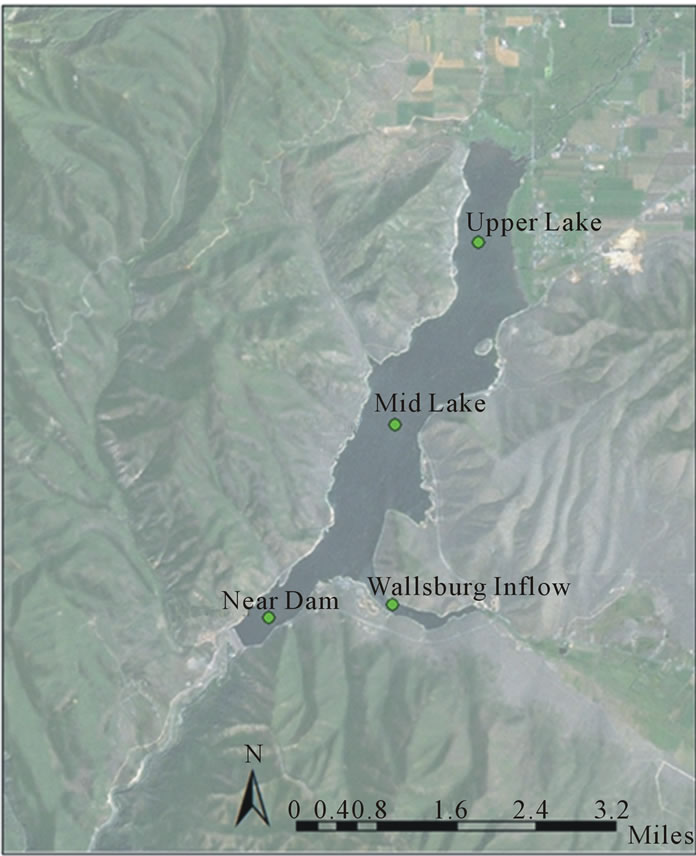
Figure 1. Sampling sites at deer creek reservoir.
trends. We selected Landsat data because of low cost and availability to download long-term historical data. Deer Creek data are acquired from Landsat paths 37 and 38, row 32 which creates a pattern of acquisition of 7-9-7 days [14]. Only images within 24 hours of the in-situ measurements were used, providing a total of 55 satellite images over the monitoring period of 1985-2005.
5. Methods
5.1. Data Processing
The Landsat images were downloaded from the USGS Earth Explorer Database. The images were calibrated, with digital numbers converted to reflectance values. The images were then atmospherically corrected using the dark subtraction algorithm in ENVI. Atmospheric correction mitigates the impacts of solar reflectance, pollution from aerosols and small particulate matter, and water vapor on the data.
5.2. Statistical Analysis
Within each satellite image, we created regions of interest using a 3 × 3 grid surrounding the location of each in-field sampling site [14,15]. A 3 × 3 grid was used to minimize image noise and spatial variation. This provides a more average measure of the reservoir condition and reflects the fact that the field data were not collected at the exact same time as the satellite data. The data for each band were averaged over the 9 pixels and the resulting mean reflectance values were assumed to represent each sampling site.
To develop the sub-seasonal models we used a regression test to compute the correlation between the two data sets (remotely sensed data and in-situ measurements). This approach requires that the data be normally distributed. We checked this assumption and found that the data for each of the spectral bands were normally distributed. However, according to the Shapiro-Wilk goodness-of-fit test, the p-value of the in-situ measurements of chlorophyll was less than 0.0001, indicating that the distribution was not normal, but the p-value for the Shapiro-Wilk test of the natural log of the in-situ measurements was 0.046, so the natural log of the in-field measured chlorophyll levels was used to provide a more normal distribution, shown in Figure 2.
We performed a stepwise linear regression analysis, evaluating combinations of each of the bands and the ratios of bands to be fit to the values of in-field measurements. Using a forward selection process, the bands and ratios of bands were included in the model until no more improvements to the model were made by the inclusion of additional data (either bands or band ratios). We created models using up to 4 variables (bands or band ratios) with a stepwise regression computed for each sub-season
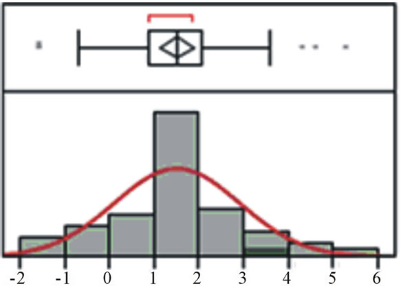
Figure 2. Distribution of ln(Chl-a) field measurements.
to produce three unique regression models for each of the three sub-seasons. Finally, we developed a model using the data set for the entire growing season to allow for comparison between sub-seasonal and an overall model.
We tested the data for the influence of outliers with the Hat, Studentized Residual, Cook’s Difference Influence tests. These tests identify the influence or leverage of univariate outliers and whether or not they should have been included in the regression analysis. The Leverage test is a measure of the distance between the predicted value and the average of the predicted values in the entire data set. An individual predicted value typically has a high potential for influence according to (1),
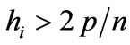 (1)
(1)
where h is the hat value, p is the number of regression coefficients, and n is the number of samples [16]. The Studentized Residual test suggests that those predicted values that are outside the range of −2 and 2 should be considered for high influence. Finally, the Cook’s Distance test analyzes the effect of omitting a case on the estimated regression coefficients. The typical cutoff for influential values is those with a distance above 1.
Only one value failed more than one test for influence and was excluded from the regression analysis. Following the exclusion of this value and a second regression analysis, the correlation coefficient was improved by 3%, and no additional data points were flagged for high influence or rejected as outliers.
6. Results
Each of the seasonal subsets of data resulted in unique models with different combinations of parameters and coefficients. The models for each of the sub-seasons are provided below (Equations 2-4). In each model, the bands are represented as BX, with X indicating the number of Landsat band.
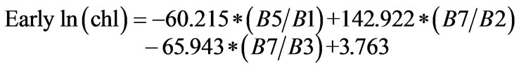 (2)
(2)
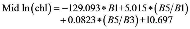 (3)
(3)
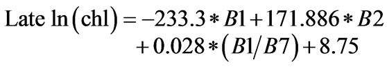 (4)
(4)
Along with the models, respective R2 values are prEsented in Table 1 to demonstrate how well the model parameters fit the data. Figure 3 presents the in-field measured chlorophyll-a versus the predicted chlorophyll-a amounts.
Additionally, a stepwise regression was performed on the entire data set. This model was then fit to the in-field measured data for the three sub-seasons. The model that was developed using only the data from the late growing season months was also applied to the earlier sub-seasons for comparison. Results of the respective actual versus predicted plots are included in Figures 4 and 5.
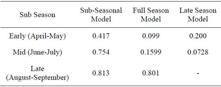
As previously discussed, the traditional modeling approach relies heavily on the data from the end of the growing season. We used the late season model to predict results in the earlier seasons. This showed that the correlation coefficient using a model developed using late summer data to predict earlier seasonal conditions was significantly lower, at R2 = 0.2 for the early-summer data and R2 = 0.0728 for the mid-summer data, indicating that a model developed using data from the later months of the growing may not accurately describe chlorophyll levels for the rest of the growing season.
The predictions for each season using the full-seasonal model (the model developed using all the data without regard for seasons) were compared against the predictions for the sub-seasonal models. The regression coefficient for the model parameters was 0.546, lower than any of the sub-seasonal models.
The correlations between actual and predicted data were also significantly lower for the earlier months of the growing season, with R2 = 0.0995 for the early season data, R2 = 0.1599 for the mid-season data. The exception was the late sub-season; however, this correlation was still lower than the individual sub-season. The comparatively poor predictive capabilities of the full season model for the earlier two sub-seasons indicate that the individual models may better describe the actual chlorophyll concentration in the reservoir.
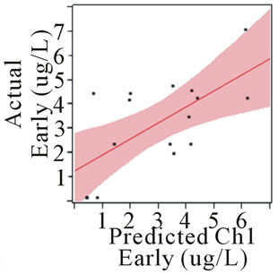 (a)
(a)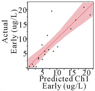 (b)
(b)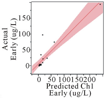 (c)
(c)
Figure 3. In-field measured values versus predicted values ((a) Early, (b) Mid, (c) Late).
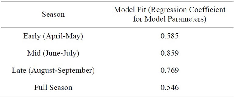
Table 1. Regression coefficients for various models.
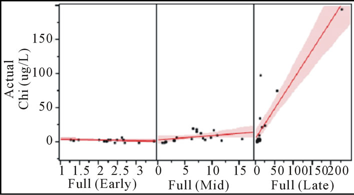
Figure 4. Actual versus predicted values for full growing season model.
7. Conclusions
The results of the regression analysis indicate that subseasonal models provide more accurate estimations of the chlorophyll levels during their respective sub-seasons than a model representing the entire growing season. Additionally, the algorithm developed for the late summer months does not provide the accuracy of the other algorithms when it is applied to the earlier months of the growing season. This indicates that sub-seasonal algo-
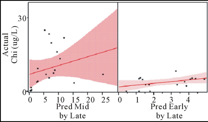
Figure 5. Actual versus predicted values for Late model applied to Early and Mid sub-seasons.
rithms may perform better and provide more accurate estimations of the chlorophyll throughout the growing season. Each of the models is unique, which indicates that the hypothesis that the different types of algae display unique visual characteristics is correct.
As Stadelmann indicated, the peak algae blooms and maximum chlorophyll levels do not always occur during the last two months of the growing season [12], so it is important to provide accurate estimations of chlorophyll throughout the growing season. These sub-seasonal models have the potential to better describe the patterns and trends of chlorophyll levels by providing more accurate remotely-sensed estimations of chlorophyll levels.
8. Acknowledgements
We thank Reed Oberndorfer and the Central Utah Water Conservancy District for providing field measurements and other data collection, the Bureau of Reclamation— Upper Colorado Region, other research group members, and the faculty and advisors in the Brigham Young University Civil and Environmental Engineering Department.
REFERENCES
- UDEQ, “Deer Creek Reservoir Lake Report,” Utah Department of Environmental Quality, 2004.
- R. W. Castenholz, “Seasonal Changes in the Attached Algae of Freshwater and Saline Lakes in the Lower Grand Coulee, Washington,” Limnology and Oceanography, Vol. 5, No. 1, 1960, pp. 1-28. http://dx.doi.org/10.4319/lo.1960.5.1.0001
- G. Prowse and J. Talling, “The Seasonal Growth and Succession of Plankton Algae in the White Nile,” Limnology and Oceanography, Vol. 3, No. 2, 1958, pp. 222-238. http://dx.doi.org/10.4319/lo.1958.3.2.0222
- T. Kutser, “Quantitative Detection of Chlorophyll in Cyanobacterial Blooms by Satellite Remote Sensing,” Limnology and Oceanography, Vol. 49, No. 6, 2004, pp. 2179-2189. http://dx.doi.org/10.4319/lo.2004.49.6.2179
- T. Kutser, L. Metsamaa, N. Strömbeck and E. Vahtmäe, “Monitoring Cyanobacterial Blooms by Satellite Remote Sensing,” Estuarine, Coastal and Shelf Science, Vol. 67, No. 1-2, 2006, pp. 303-312. http://dx.doi.org/10.1016/j.ecss.2005.11.024
- S. A. Spaulding and L. Elwell, “Increase in Nuisance Blooms and Geographic Expansion of the Freshwater Diatom Didymosphenia Geminate,” 2007.
- EPA, “Confirmed Presence of D. geminata in the United States and Canada.” www.epa.gov/region8/water/didymosphenia
- S. Sathyendranath, L. Watts, E. Devred, T. Platt, C. Caverhill and H. Maass, “Discrimination of Diatoms from Other Phytoplankton Using Ocean-Colour Data,” Marine ecology Progress Series, Vol. 272, 2004, pp. 59-68. http://dx.doi.org/10.3354/meps272059
- D. C. Rundquist, L. Han, J. F. Schalles and J. S. Peake, “Remote Measurement of Algal Chlorophyll in Surface Waters: The Case for the First Derivative of Reflectance near 690 nm,” Photogrammetric Engineering and Remote Sensing, Vol. 62, 1996, pp. 195-200.
- S. Mishra and D. R. Mishra, “Normalized Difference Chlorophyll Index: A Novel Model for Remote Estimation of Chlorophyll-< i> a Concentration in Turbid Productive Waters,” Remote Sensing of Environment, 2011.
- D. A. Fayol, “Evaluation of the TMDL for the East Canyon Reservoir Using Remote Sensing,” Master of Science Thesis, Department of Civil and Environmental Engineering, Brigham Young University, 2011.
- T. H. Stadelmann, P. L. Brezonik and S. Kloiber, “Seasonal Patterns of Chlorophyll a and Secchi Disk Transparency in Lakes of East-Central Minnesota: Implications for Design of Ground-and Satellite-Based Monitoring Programs,” Lake and Reservoir Management, Vol. 17, No. 4, 2001, pp. 299-314. http://dx.doi.org/10.1080/07438140109354137
- K. E. Sawaya, L. G. Olmanson, N. J. Heinert, P. L. Brezonik and M. E. Bauer, “Extending Satellite Remote Sensing to Local Scales: Land and Water Resource Monitoring Using High-Resolution Imagery,” Remote Sensing of Environment, Vol. 88, No. 1-2, 2003, pp. 144-156. http://dx.doi.org/10.1016/j.rse.2003.04.006
- C. Giardino, M. Pepe, P. A. Brivio, P. Ghezzi and E. Zilioli, “Detecting Chlorophyll, Secchi Disk Depth and Surface Temperature in a Sub-Alpine Lake Using Landsat Imagery,” Science of the Total Environment, Vol. 268, No. 1-3, 2001, pp. 19-29. http://dx.doi.org/10.1016/S0048-9697(00)00692-6
- S. W. Bailey and P. J. Werdell, “A Multi-Sensor Approach for the On-Orbit Validation of Ocean Color Satellite Data Products,” Remote Sensing of Environment, Vol. 102, No. 1-2, 2006, pp. 12-23. http://dx.doi.org/10.1016/j.rse.2006.01.015
- F. L. Ramsey and D. W. Schafer, “The Statistical Sleuth: A Course in Methods of Data Analysis,” 2nd Edition, Cengage Learning, 2002.