International Journal of Clean Coal and Energy
Vol.2 No.3(2013), Article ID:36046,19 pages DOI:10.4236/ijcce.2013.23005
Implementation of a Demoisturization and Devolatilization Model in Multi-Phase Simulation of a Hybrid Entrained-Flow and Fluidized Bed Mild Gasifier
Energy Conversion & Conservation Center, University of New Orleans, New Orleans, USA
Email: jrkhan@uno.edu, twang@uno.edu
Copyright © 2013 Jobaidur Khan, Ting Wang. This is an open access article distributed under the Creative Commons Attribution License, which permits unrestricted use, distribution, and reproduction in any medium, provided the original work is properly cited.
Received March 23, 2013; revised April 23, 2013; accepted May 1, 2013
Keywords: Multi-Phase Simulation; Gasification Simulation; Entrained-Flow Gasifier; Fluidized Bed Mild Gasifier; Clean Coal Technology
ABSTRACT
A mild gasification process has been implemented to provide an alternative form of clean coal technology called the Integrated Mild Gasification Combined Cycle (IMGCC), which can be utilized to build a new, highly efficient, and compact power plant or to retrofit an existing coal-fired power plant in order to achieve lower emissions and significantly improved thermal efficiency. The core technology of the mild gasification power plant lies on the design of a compact and effective mild gasifier that can produce synthesis gases with high energy volatiles through a hybrid system: utilizing the features of both entrained-flow and fluidized bed gasifiers. To aid in the design of the mild gasifier, a computational model has been implemented to investigate the thermal-flow and gasification process inside this mild gasifier using the commercial CFD (Computational Fluid Dynamics) solver ANSYS/FLUENT. The Eulerian-Eulerian method is employed to model both the primary phase (air) and the secondary phase (coal particles). However, the Eulerian-Eulerian model used in the software does not facilitate any built-in devolatilization model. The objective of this study is therefore to implement a devolatilization model (along with demoisturization) and incorporate it into the existing code. The Navier-Stokes equations and seven species transport equations are solved with three heterogeneous (gassolid) and two homogeneous (gas-gas) global gasification reactions. Implementation of the complete model starts from adding demoisturization first, then devolatilization, and then adding one chemical equation at a time until finally all reactions are included in the multiphase flow. The result shows that the demoisturization and devolatilization models are successfully incorporated and a large amount of volatiles are preserved as high-energy fuels in the syngas stream without being further cracked or reacted into lighter gases. The overall results are encouraging but require future experimental data for verification.
1. Introduction
Coal has been widely utilized to produce electric power. Approximately 49 percent of electricity in the United States is produced by coal up to 2012. Unfortunately coal is dirty: burning coal releases large amounts of greenhouse gases (CO2 and NOx) and other pollutants such as SOx, soot, mercury, and ash. Therefore, it is essential to continuously develop new technologies to utilize coal more cleanly. The method of using coal can be categorized into four main processes: 1) combustion, 2) pyrolysis, 3) liquefaction, and 4) gasification. This study is focused on gasification technology.
1.1. Coal Gasification
Figure 1 presents the typical stages of coal gasification. The gasification of coal particles involves three major steps: 1) thermal decomposition (pyrolysis and devolatilization), 2) thermal cracking of the volatiles, and 3) char gasification. Coal particles undergo pyrolysis when they enter the hot combustion environment. Moisture within the coal boils and leaves the coal’s core structure when the particle temperature reaches the boiling point. The volatiles are then released as the particle temperature continues to increase. This volatile-releasing process is called devolatilization. The long hydrocarbon chains are
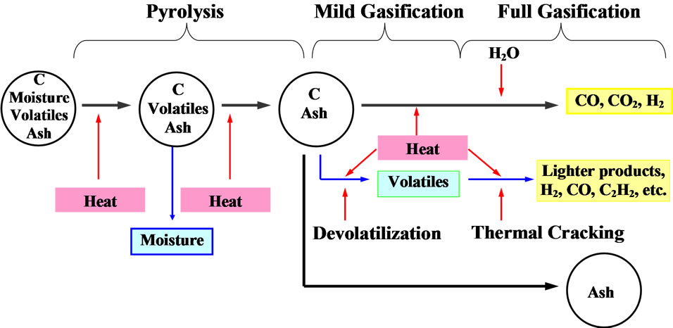
Figure 1. Simplified global gasification processes of coal particles (sulfur and other minerals are not included in this figure).
then thermally cracked into lighter volatile gases, such as H2, CO, C2H2, C6H6, CH4, etc. These lighter gases can react with O2, releasing more heat, which is needed to continue the pyrolysis reaction.
With only char and ash left, the char particles undergo gasification with CO2 or steam to produce CO and H2, leaving only ash. The heat required for the pyrolysis and devolatilization processes can be provided externally or internally by burning the char and/or volatiles.
1.2. Devolatilization
Devolatilization is a decomposition process that occurs when volatiles are driven out from a hydrocarbon material (like coal) under heating. The rate of devolatilization is influenced by temperature, residence time, particle size, and coal type. The heating causes chemical bonds to rupture and both the organic and inorganic compounds to decompose. The process starts at a temperature of around 100˚C (212˚F) with desorption of gases, such as water vapor, CO2, CH4, and N2, which are stored in the coal pores. When the temperature reaches above 300˚C (572˚F), the released liquid hydrocarbon called tar becomes important. Gaseous compounds, such as CO, CO2, and steam are also released. When the temperature is above 500˚C (932˚F), the fuel particles are in a plastic state, through which they undergo drastic changes in size and shape. The coal particles then harden again and become char when the temperature reaches around 550˚C (1022˚F). Heating continues, H2 and CO are released through gasification.
The pyrolysis conditions affect the physical properties of the char. It is reported that the heat transfer coefficient decreases by a factor of 10 during the fast heating of the coal particles mixed with a hot solid heat carrier. This reduced heat transfer rate to the particle surface results in a temperature plateau on the level of about 400˚C (752˚F) and lasts throughout the devolatilization process.
In general, the larger the particle size, the smaller the volatiles yield. This is because, in larger particles, more volatiles may crack, condense, or polymerize, with some carbon deposition occurring during their migration from inside the particle to the particle surface. High pressure has a similar effect on the devolatilization rate. Anthony et al. [1] reported that devolatilization rates are higher at lower pressures. An increase in pressure increases the transit time of volatiles rising to the particle surface.
1.3. Types of Gasifiers
There are many types of gasifiers. The operating principles of two commonly used gasifiers (the entrained-flow and fluidized bed gasifier) are used in designing the studied mild gasifier, so only these two types of gasifiers are briefly introduced below:
1.3.1. Entrained-Flow Gasifier
In the entrained-flow gasifier, a dry, pulverized coal, an atomized liquid fuel, or a fuel slurry is gasified with oxygen (much less frequent: air) in a flow at a speed of 10 - 15 m/s under an operating pressure ranging from 1 to 60 atm. The gasification reactions take place in a dense cloud of very fine particles. Most coals are suitable for this type of gasifier because of the high operating temperatures and the high heat transfer rates to the individual particles, resulting from the fact that the coal particles are well separated from one another. All entrained-flow gasifiers remove the major part of the ash as slag because the operating temperature is typically well above the ash fusion temperature. A smaller fraction of the ash is produced either as a very fine fly ash or as a black ash slurry. The merit of an entrained flow gasifier is its high mass flow rate and high product yield.
1.3.2. Fluidized Bed Gasifier
In a fluidized bed gasifier, air or oxygen is injected upward at the bottom of a solid fuel bed, suspending the fuel particles. The fluidized bed acts like a multiphase, granular flow field. The fuel feed rate and the gasifier temperature are lower compared to those of entrainedflow gasifiers. The operating temperature of a fluidized bed gasifier is also lower: around 1000˚C (1830˚F), which is roughly only half of the operating temperature of a coal burner. This lower temperature has several advantages: lower NOx emissions, no slag formation, and low syngas temperature, which can result in a cheaper syngas cooling system being used prior to gas clean up, meaning higher cycle efficiency. Fluidized bed gasifiers require a moderate supply of oxygen and steam.
1.4. Complete, Partial, Full, and Mild Gasification
For clarification, the terms of full, partial, and mild gasification are defined below:
Complete and Partial gasification describe how much char is left unreacted. Complete Gasification implies that all the char is completely gasified, while Partial Gasification indicates that a portion of the char remains unreacted. The carbon conversion rate (CCR), also called carbon conversion efficiency, represents the fraction of carbon reacted and formulated as:
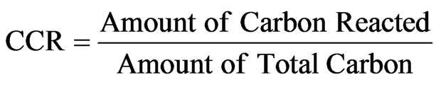 (1)
(1)
Full and Mild gasification describe the level (i.e., the products’ molecular weight or length of molecular chain) of thermal cracking, which is typically affected by the temperature level and residence time of reaction. Full Gasification indicates that the feedstock undergoes complete de-volatilization, gasification, and thermal cracking into a composition consisting of light species like CO, H2, and CH4 as the major combustible components of the socalled syngas, while Mild Gasification preserves the heavier volatiles without further thermally cracking them into lighter components. To be specific, the operation of “Mild Gasification” refers to controlling the temperature and residence time to achieve varying levels of gasification between pyrolysis-only (0% gasification) and full gasification (100% gasification). It is a comprehensive process to design such a gasifier that can control the level of thermal cracking that occurs.
1.5. Hydrodynamics of Fluidized Beds
The simulated mild gasifier is unique in its hybrid characteristics with both entrained-flow and fluidized bed features, so no similar CFD study has been performed before in this type of mild gasifier. The closest simulation will be those numerical analyses performed for a fluidized bed gasifier. A literature review is hereby provided below.
Ergun [2] critically reviewed and studied the exiting information on the flow of fluids through beds of granular solids. He reported experimental results obtained for the purpose of testing the validity of the equation and numerous other data taken from the literature. He found that pressure losses are caused by simultaneous kinetic energy and viscous energy losses. He examined the dependence of pressure upon flow rate, properties of the fluids, and fractional void volume (ε), as well as the orientation, size, shape, and surface of the granular solids.
Syamlal and Gidaspow [3] developed a computer model for a hot fluidized bed for gasifying coal due to high rates of heat and mass transfer and solids mobility. Syamlal [4] developed a multi-particle model of fluidization. He simulated fluidization phenomena such as segregation, elutriation, and solids mixing. He derived an expression for the particle-particle drag term based on the kinetic theory of dense gases. He also compared the predictions of the model with Yang and Keairns’s [5] experimental data to test the accuracy of that expression. Yang and Keairns fluidized uniform mixtures of dolomite and acrylic particles for various times and they also measured the rate of separation of the dolomite particles from the acrylic particles. Yang and Keairns’s experimental data suggest that the rate of settling is strongly dependent upon the particle-particle drag. Yang and Keairns experiments provided useful information to more accurately determine the particle-particle drag term.
Syamlal and O’Brien [6] studied bubble behavior. They used a hydrodynamic model to treat a fluidized medium as a mixture of a gas and a granular (solid) phase. They simulated the bubbles in fluidized beds of various particle sizes, with and without jets. They found that the predicted characteristics of bubble formation, bubble shape, bubble coalescence phenomena, bubble motion, bubble eruption at the surface, and the dynamics of the bed surface are in good qualitative agreement with experimental observations.
Gunn [7] measured the experimental heat transfer to particles in fixed beds and showed that either the Nusselt number remains constant as the Reynolds number is reduced or the Nusselt number decreases to zero if axial dispersion has been neglected. A quantitative analysis of particle to fluid heat transfer based on a stochastic model of the fixed bed leads to a constant value of the Nusselt group at low Reynolds numbers. When the analytical equation is included as an asymptotic condition, he derived an expression that describes the dependence of the Nusselt group upon the Reynolds number. He extended this expression to describe mass and heat transfer to fixed and fluidized beds of particles within the porosity range of 0.35 to 1.0. Both the gas and liquid phase transfer groups are correlated up to a Reynolds number of 105.
Lun et al. [8] studied the flow of an idealized granular material consisting of uniform, smooth but inelastic, spherical particles using statistical methods analogous to those used in the kinetic theory of gases. They developed two theories: one for the Couette flow of particles having arbitrary coefficients of restitution (inelastic particles) and a second for the general flow of particles with coefficients of restitution near one (slightly inelastic particles). The study of inelastic particles in Couette flow follows the method of Savage and Jeffrey [9]. An ad hoc distribution function was used to describe the collisions between particles. They compared the results of this first analysis with other theories of granular flow, with the Chapman-Enskog dense-gas theory, and with experiments. Their theory agreed moderately well with experimental data.
Kuipers et al. [10] developed a computational model for a hot gas-fluidized bed. They used the two-fluid model (TFM) approach. In that approach both phases are considered to be continuous and fully interpenetrating. They calculated local wall-to-bed heat transfer coefficients by simultaneously solving the two-fluid model (TFM) conservation of mass, momentum and energy equations. Their preliminary calculations suggest that the experimentally observed high wall-to-bed heat transfer coefficients of gas-fluidized beds can be predicated with the present hydrodynamic model without the incorporation of turbulence terms in the transport equation.
Enwald et al. [11] carried out a mesh refinement study and validation of two-fluid model closures for a bubbling fluidized bed application. The mesh refinement study indicates that a higher degree of mesh refinement is required for atmospheric than for pressurized fluidization. They computed the simulated statistical bubble quantities from voidage signals derived from the transient multidimensional solution of two-fluid models. They developed a parallel version of the two-fluid model solver to remedy the long simulation times required to obtain acceptable statistical values, based on a domain decomposition method for distributed memory computers.
Jiradilok et al. [12] studied the turbulent fluidization regime, which is characterized by the co-existence of a dense, bottom region and a dilute, top bed. A kinetic theory-based CFD code including a drag model for clusters captured the basic features of this flow regime: the dilute and dense regions, high dispersion coefficients, and strong anisotropy. The computed turbulent kinetic energy is close to the measurements for Fluidized Catalytic Cracking (FCC) particles. The computed solid pressures, granular temperatures, FCC viscosities, and frequencies of oscillations were close to the measurements reported in the literature.
Panneerselvam et al. [13] carried out CFD simulations for the prediction of flow patterns in a liquid-solid fluidized bed using the Eulerian-Eulerian framework. They compared the CFD model predictions with the experimental findings. They further extended the CFD model to compute solid mass balance in the core and annular regions for verifying conservation of mass and energy flows due to various dissipation mechanisms. They also compared energy required for solid expansion in liquid fluidized bed with energy required for solid suspension in an equivalent stirred tank contactor at similar operating conditions. They investigated the influence of various inter-phase drag models on solids in liquid fluidized beds.
Reuge et al. [14] validated a CFD model that they used for designing fluidized bed reactors. They collected the validation data from a fluidized bed of alumina particles operated at different gas velocities involving two fluidization hydrodynamic regimes (bubbling and slugging). They measured the bed expansion, height of bed fluctuations, and frequency of fluctuations from videos of the fluidized bed. To simulate the experiments they used the Eulerian-Eulerian two fluid models using an open-source code MFiX (Multiphase Flow with Interphase eXchanges) [15], which is a general-purpose computer code developed at the National Energy Technology Laboratory (NETL) of the US Department of Energy for describing the hydrodynamics, heat transfer, and chemical reactions in fluid-solid systems.
1.6. Simulation of Reactions in Fluidized Beds
Chejne and Hernandez [16] developed a one-dimensional steady-state mathematical model and a numerical algorithm to simulate the coal gasification process in a fluidized-bed using FORTRAN 90. The model incorporates two phases, the solid and the gas, for instantaneous coal devolatilization. Their model could predict temperature, species mole fractions, and particle size distribution for the solid phase.
Yu et al. [17] developed a numerical model based on the two-fluid model (TFM,) including the kinetic theory of granular flow (KTGF) and chemical reactions to simulate coal gasification in a bubbling fluidized bed gasifier (BFBG.) They modeled instantaneous coal devolatilization. They determined the coal gasification rates by combining the Arrhenius rate and diffusion rate for heterogeneous reactions and using the turbulent mixing rate for homogeneous reactions. The flow behaviors of the gas and solid phases in the bed and freeboard were obtained from the analysis. The calculated exit values of the gas composition agreed well with the experimental data.
Wang, Jin, and Zhong [18] developed a comprehensive three-dimensional numerical model to simulate the coal gasification in a fluidized bed gasifier. They considered both gas-solid flow and chemical reactions. They modeled the gas phase with k-ε turbulent model and the particle phase with kinetic theory of granular flow. Their analysis considered the coal pyrolysis, homogeneous reactions and heterogeneous reactions. The predicted exit gas compositions were in a good agreement with the experiments.
Most of the previous researchers modeled instantaneous devolatilization. Suo-Anttila et al. [19] described a new Large Eddy Simulation (LES) based CFD code to simulate multiphase coal and biomass combustion and gasification in a transient Eulerian framework. They have added a sub-model to approximate coal/biomass devolatilization and char oxidation. They modeled the devolatilization in different stages in detail.
2. Motivation and Objective
The sole function of all of the gasifiers used for electrical power generation is to produce syngas, consisting of light gases such as CO, H2, and CH4 as the major fuels. The major reason for wanting to produce light gases is to avoid condensation of tars or heavy volatiles in the gas cleaning systems, which are usually operated at temperatures lower than the volatiles' dew points. Therefore, if gas cleaning can be performed at a temperature higher than the volatiles’ dew points, it becomes interesting to investigate the feasibility of producing mildly-gasified syngas with a large portion of this syngas consisting of heavier volatiles with higher energy density to save the energy consumed for thermally cracking the volatiles into lighter gases.
The recent successful development of a pilot gas cleanup system by RTI International in Eastman’s coal gasification facility in Kingsport, Tennessee with support from the US Department of Energy [20] provides the necessary technology breakthrough to utilize the mildlygasified syngas studied in this paper. This system could remove sulfur, ammonia, mercury, arsenic, selenium, and chlorine at temperatures between 600˚F and 1000˚F. The goal is to get the operating temperature above 1000˚F— this is the temperature above which almost all the volatiles will remain in the vapor phase. The RTI warm gas clean up system has been incorporated into the Polk Power Station IGCC plant in Tampa, Florida for commercial testing [21].
Implementing the mild-gasification concept to an IGCC system is conceptually shown as an integrated mild-gasification combined cycle (IMGCC) in Figure 2. Note that IMGCC is different from the conventional Partial Gasification system, which also uses a gasifier to produce the char but the latter uses a large amount of energy to thermally crack the volatiles fully to lighter gases, rather than preserve the volatiles and gases with higherenergy densities, as the former does.
In addition to the energy savings, there are several other attractive advantages for using mildly-gasified syngas: since a typical mildly-gasified syngas contains approximately 6 times more energy than a fully-gasified syngas, the sizes of the mild gasifier and gas cleaning systems can be shrunk down by about 80%. Then, the remaining unreacted char can be used in the boiler of a conventional pulverized coal (PC) power plant with negligible sulfur content (see Figure 2). This advantage leads to the possibility of using mild gasification technology to retrofit existing PC power plants by replacing the coal feedstock with the char produced by a mild gasifier.
The mildly-gasified syngas can be burned in the gas turbine combustor after it goes through the gas cleaning systems. The exhaust of the gas turbine can produce steam via a heat recovery steam generator (HRSG) to produce steam to generate electricity via a steam turbine, like a traditional combined cycle. Only this time, the steam produced by the HRSG is mixed with the steam produced with the boiler of the existing PC plant operated in a Rankine cycle. This retrofit can significantly increase the plant efficiency from about 30% to 50% (HHV) as well as drastically reduce the emissions per kW output because the syngas can be cleaned before combustion more economically than is possible after combustion due to the low volume flow rate of mild-
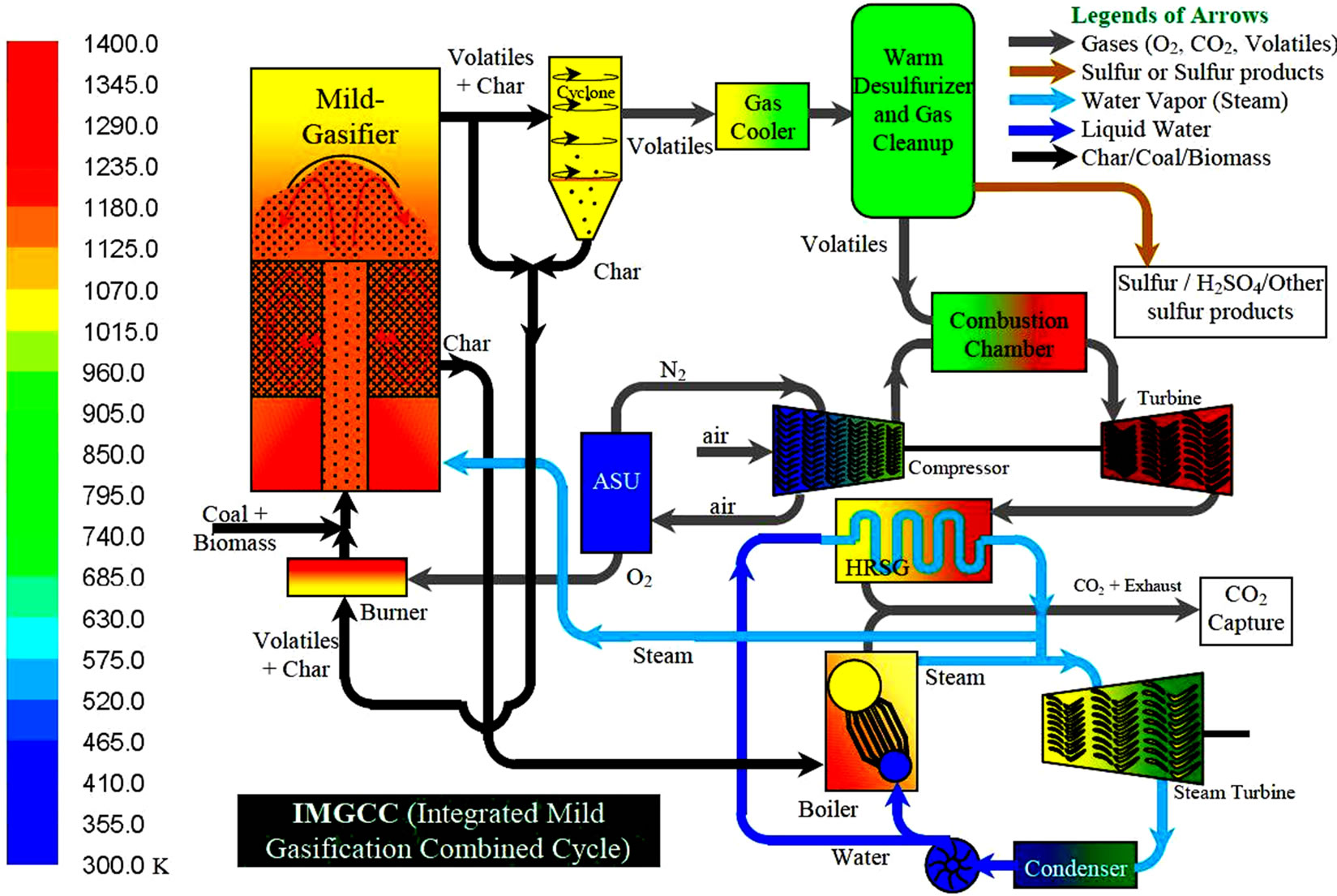
Figure 2. A system diagram of an integrated mild-gasification combined cycle (IMGCC).
gasified syngas and increased overall cycle efficiency. Furthermore, the scrubber of the original PC plant could be minimized or removed, reducing the overall plant operating and maintenance (O & M) cost.
This approach was first proposed by Wormser as the Mild Air-Blown Gasification Integrated Combined Cycle (MaGIC) [22,23]. However, in MaGIC, the gasifier is operated under the air-blown condition without using an air separation unit (ASU); whereas in an IMGCC system, either air-blown or oxygen-blown operation can be implemented. The core technology of the mild-gasification power plant is a compact and effective mild gasifier that can control the level of thermal cracking that occurs. This need motivates the research at the Energy Conversion and Conservation Center (ECCC) to design a conceptual laboratory scale gasifier. To help design this mild gasifier, a computational model is to be implemented to investigate the thermal-flow, devolatilization, and gasification process inside this mild gasifier using the commercial CFD solver ANSYS/FLUENT. Eulerian-Eulerian method is employed to model both the primary phase (air) and the secondary phase (coal particles). However, the Eulerian-Eulerian model in the used software does not facilitate any built-in devolatilization model. The objective of this study is therefore to implement a devolatilization model (along with a demoisturization model) and incorporate it into the existing code. This is an Eulerian-Eulerian model that works with volume fraction. This model will be called successful if the moisture and volatile fraction can be reduced in coal but increase in the same amount in gas mixtures. The actual demoisture and devolatilization rates are not included in the evaluation of success in the paper until experimental data is available for validation in the future.
3. Description of the Studied Mild Gasifier
The conceptual design of a 100 kW, laboratory scale mild gasifier, as shown in Figure 3, is a hybrid system which combines features of both an entrained-flow and a fluidized bed gasifier. The entrained-flow feature is characterized by the centralized draft tube. Through the drafttube’s bottom inlet, coal and a limited amount of oxidant (air or oxygen) are introduced to produce heat, which is used to drive out the volatiles during the journey upward through the draft tube. Surrounding the draft tube is the fluidized bed. The draft tube is 4 inches (10.15 cm) in diameter to prevent the volatiles inside from contacting the oxygen in the fluidization air in the fluidized bed, but this setup allows heat to be transferred from the draft tube to the fluidized bed through the draft tube wall. Above the draft tube, a deflector 8 inches in diameter is installed to block the particles from being entrained out of the fluidized bed. The height and width of the benchtop mild gasifier is 34.25 inches (87 cm) and 18 inches
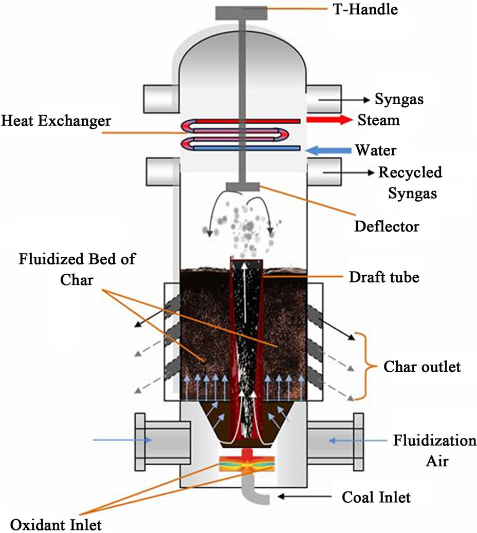
Figure 3. Schematic diagram of the cold-flow model of the conceptual Mild Gasifier, a variation derived from Wormser’s design [22].
(45.75 cm), respectively.
There are three velocity inlets, two for the fluidization gas and one for the coal and transport gas. The diameter of the left and right horizontal gas inlets is 3 inches (7.65 cm) and the vertical coal inlet is 2 inches (5 cm) in diameter. There are four outlets, two for char and two for the produced syngas. The diameter of the left and right horizontal syngas outlets is 5 inches (12.7 cm) and the char outlets are 1.5 inches (3.8 cm,) inclined 45 degrees. To determine the most effective location to extract desired chars, three pairs of inclined char chutes are designed in the test model, although only one pair will be used for each experiment. The fluidized bed is 10 inches (0.254 m) deep. To create fluidization inside the gasifier, a total of 28 perforated interior surfaces, 0.15 inches (0.38 cm) in diameter each, are created side by side, equally spaced.
4. Computational Model
CFD is an economical and effective tool to study coal gasification. Coal gasification is a multiphase reactive flow phenomenon: it is a multiphase problem between gases and coal particles and also a reactive flow problem, which involves homogeneous reactions among gases and heterogeneous reactions between coal particles and gases. The Eulerian-Eulerian method is adopted in this study because the concentrations of coal particles are dense in the fluidized bed and tracking each particle with the Lagrangian method is not realistic given current computational capability. Although, inside the draft tube, the conditions are similar to an entrained-flow gasifier, so the Lagrangian-Eulerian method could be used here. However, since the Lagrangian-Eulerian method can’t be used to obtain a solution within the fluidized bed, while Eulerian-Eulerian can be used in both the entrained-flow and fluidized bed portions of the gasifier, the EulerianEulearian method is adopted in this study. This means that both the gas phase (primary phase) and solid phase (secondary phase) are solved by using the Eulerian method.
The solid particles are placed in the domain of the fluidized bed like a bed of granular material. The mixture of the gas phases of different species passes through this bed and converts this granular material from a static, solid-like state to a dynamic, fluid-like state. This process is known as “fluidization”. Both homogeneous (gasgas) reactions and heterogeneous (gas-solid) reactions are simulated in this study. The central-plane geometry of the 2-D Mild Gasifier used in the simulation is shown in Figure 4.
4.1. Model Characteristics of the Problem
The physical characteristics of the problem are modeled as follows:
1) The flow inside the domain is two dimensional, incompressible, and turbulent.
2) The gravitational force is considered.
3) Gas species involved in this study are Newtonian fluids with variable properties as functions of temperature. These variable properties are calculated by using a piecewise-polynomial method.
4) A mass-weighted mixing law for specific heat and the incompressible, ideal gas law for density are used for gas species mixtures.
5) All of the outside walls are impermeable and adiabatic, but the draft tube’s wall is set as a “coupled” condition with zero thickness (called “shell wall”) so the heat transfer can be computed across the shell wall by imposing the same heat flux on both sides of the wall.
6) The no-slip condition (zero velocity) is imposed on all wall surfaces.
4.2. Multiphase Flow Regimes
In the Eulerian-Eulerian approach, the different phases are treated mathematically as interpenetrating continua. The concept of a phasic volume fraction is introduced in this approach. These volume fractions are assumed to be continuous functions of space and time and their sum is always equal to one. For each phase, conservation equations are derived to obtain a set of equations which have a similar structure for all phases. These equations are closed by providing constitutive relations that are ob-
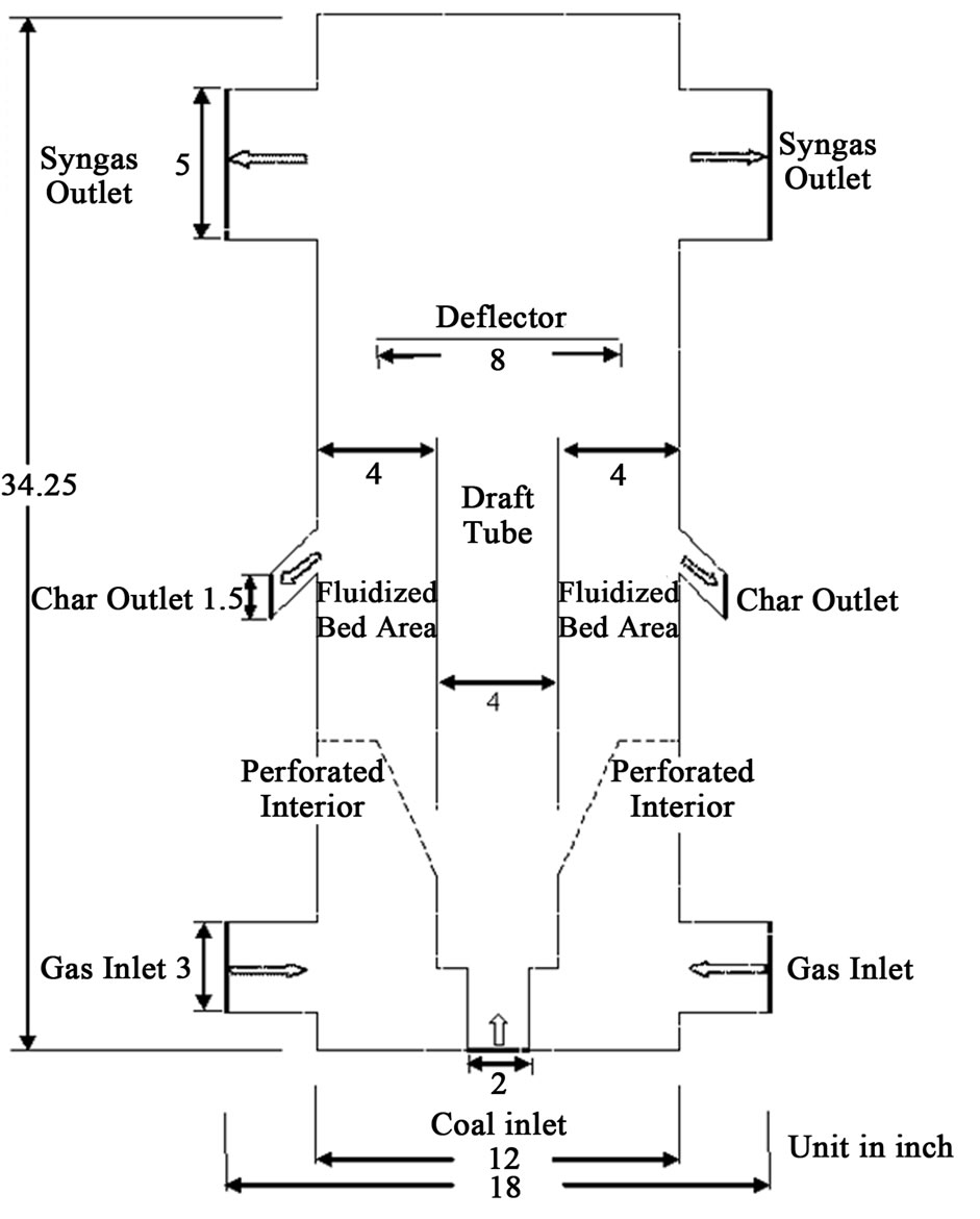
Figure 4. Schematic of the 2D simulated Mild Gasifier.
tained from empirical information, or, in the case of granular (solid) flows, by application of kinetic theory.
Two phases are considered: the primary phase (referred to as the gas phase,) which consists of all gases, e.g. O2, N2, H2, CO, CO2, H2O vapor, C6H6, and volatiles; and the secondary phase (referred to as the coal phase), which consists of char (pure carbon), H2O vapor, and volatiles. The devolatilization model (proposed in this study) disengages the H2O vapor and the volatiles from the coal phase and places them into the gas phase. A detailed description of the devolatilization model implementation is shown later.
The Eulerian model allows for the modeling of multiple, separate, interacting phases. It solves a set of “n” momentum and continuity equations for each phase, where n is the number of phases. The pressure and interphase exchange coefficients are coupled in this model. The involved equations for solving multiphase flows are extensive; only the major governing equations are selectively presented below. A more detailed description of constitutive equations, effective property values of granular flows, and interfacial dynamics and reactions is referred to papers by Mazumder and Wang [24] or Mazumder, et al. [25,26].
4.3. Governing Equations
The unsteady equations for conservation of mass, momentum, and energy using the Eulerian multiphase model are presented below:
The continuity equation for phase “q” is
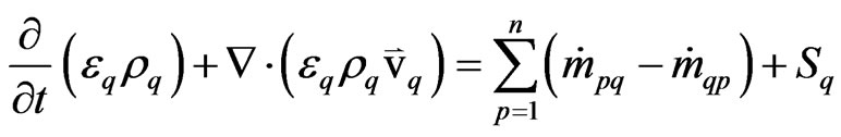 (2)
(2)
where,  = the velocity of phase “q”;
ρq = the density of phase “q”;
 = the mass transfer from phase “p” to phase “q”;
 = the mass transfer from phase “q” to phase “p”;
εq = the volume fraction of phase “q”;
Sq = the source term of phase “q”.
The momentum balance for phase “q” is
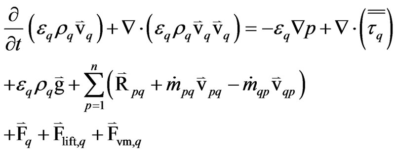 (3)
(3)
where,  , is the stress-strain tensor of phase “q” given by
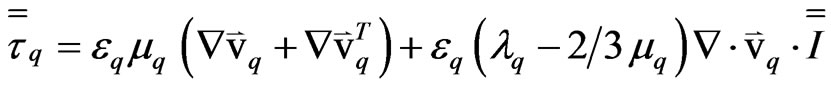 (4)
(4)
 = Inter-phase force,
  depends on the friction, pressure, cohesion, and other effects.
mq = the shear viscosity of phase “q”;
lq = the bulk viscosity of phase “q”;
 = an external body force of phase “q”;
 = lift force acting on a secondary phase “p” in a primary phase;
 = inertia of the primary phase mass encountered by the accelerating particles or droplets or bubbles exerted by a “virtual mass force” on the particles.
Ñp = the pressure gradient shared by all phases.
 = the inter-phase velocity between the phase p and q.
 = acceleration due to gravity.
One of the major differences between the single phase momentum equation and the Eulerian multiphase momentum equation is the inter-phase momentum exchange coefficient. For a solid phase “s” the conservation of momentum equation is
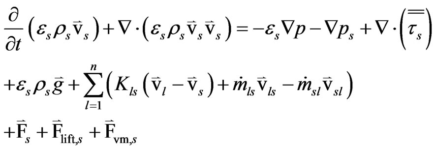 (5)
(5)
where, ps = the solid pressure of the solid phase “s”.
To describe the conservation of energy in the Eulerian multiphase model, a separate enthalpy equation is written for each phase:
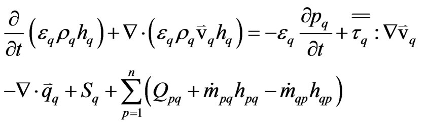 (6)
(6)
where, hq = the specific enthalpy of the phase “q”.
Qpq = the rate of heat transfer between the phase “p” and “q”.
hpq = the inter-phase enthalpy transfer between the phase “p” and “q”.
4.4. Devolatilization Model
Devolatilization is a process where moisture and volatile matters are driven out from coal by heat. The devolatilization rate (DR) represents the fraction of volatiles released from coal per unit time, expressed as:
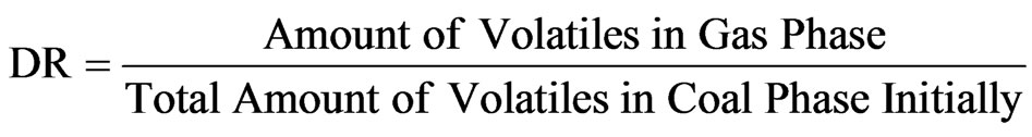 (7)
(7)
To adequately simulate the mild-gasification process, an appropriate devolatilization process is more important than simulating the full-gasification process. Since no devolatilization process is available in ANSYS/FLUENT for the Eulerian/Eulerian method (although built-in devolatilization models are available for the LangrangianEulerian method), it is necessary to incorporate a devolatilization model into the computational code as the first priority for simulating the mild-gasification process.
Four traditional devolatilization models have been commonly employed and are briefly introduced below. They are the Kobayashi, single rate, constant rate, and Chemical Percolation Devolatilization (CPD) models.
In the Kobayashi model [27], two competing devolatilization rates are expressed as a weighted function of two competing rates, k1 and k2, as:
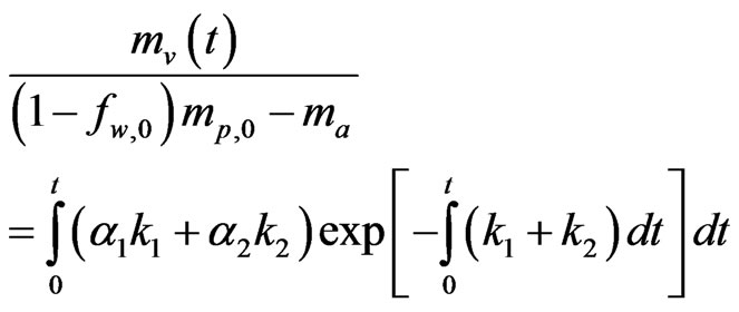 (8)
(8)
where, a1 and a2 are yield factors, fw is the mass fraction of moisture, mp is the mass of a particle, ma is the mass of ash, and k1 and k2 are given as:
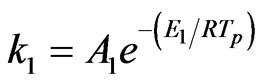 (9)
(9)
and
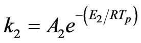 (10)
(10)
The value of the constants are A1 = 2 ´ 105, A2 = 1.3 ´ 107, E1 = 1.046 ´ 108 J/kmol, and E2 = 1.67 ´ 108 J/kmol.
The single rate model was introduced by Badzioch and Hawsley [28]. They modeled the devolatilization rate as dependent on the amount of volatiles remaining in coal following the Arrhenius form:
 (11)
(11)
where, A = pre-exponential factor = 4.92 ´ 105 and, E = activation energy = 7.4 ´ 107 J/kmol.
Baum and Street [29] modeled devolatilization assuming a constant rate. Pillai [30] used 12/s in his study.
Fletcher et al. [31,32] and Grant et al. [33] developed the Chemical Percolation Devolatilization (CPD) model by considering the chemical transformation of the coal structure during devolatilization. It models the coal structure transformation as a transformation of the chemical bridge network, which results in the release of light gas, char, and tar.
These four devolatilization models were compared by Silaen and Wang [34] in simulating gasification processes in a two-stage, entrained-flow coal gasifier by using the Eulerian-Langrangian approach. They concluded that the Kobayashi model produces a slower devolatilization rate than the other models, while the constant rate model produced the fastest devolatilization rate. The single rate model and the CPD model produced moderate and consistent devolatilization rates, however, the CPD model required more computational time. Following Silaen and Wang’s conclusion, the single rate model is adopted in this study. Implementation of the CPD model will be conducted in a future study.
In this study, devolatilization is modeled in two steps as shown in Figure 1. Firstly, the coal releases moisture during the demoisturization process and then it releases volatile matters. Based on the coal composition, the volatile in this study is chemically formulated as CH2.121O0.585. Two pseudo-heterogeneous reactions modeled with a single reaction rate in the Arrhenius form are introduced here to model these two steps. The two Eulerian-Eulerian phases assigned in this study are the primary gas phase (phase 1) and the secondary solid coal phase (phase 2). The primary phase contains all gases including O2, N2, H2O (g), CO, CO2, H2, C6H6 and volatiles, and the secondary phase contains Char (solid carbon), H2O (l) and condensed volatiles. Initially, the primary phase does not contain any water vapor (H2O) or volatiles and the secondary phase contains liquid water and condensed volatiles according to the coal composition. As devolatilization (along with demoisturization) continues, the secondary phase starts to lose moisture and volatiles, and, in the meantime, the primary phase starts to gather water vapor and volatiles. These two pseudo-chemical reactions are formulated as:
Phase 2 in coal: H2O ® Phase 1in gas: H2O (12)
Phase 2 in coal: CH2.121O0.585 ® Phase 1 in gas: CH2.121O0.58 (13)
The activation energies (4th column in Table 1) for Equations (12) and (13) are calculated by trial and error based on devolatilization time experienced in entrained flow gasifies. The trial starts from employing the single rate (Equation (4)) proposed by Badzioch and Hawsley [28].
4.5. Chemical Reaction Model
In the finite-rate model, the chemical reactions (shown in Table 1) involve both homogeneous (gas-gas) and heterogeneous (solid-gas) reactions. Reaction rates based on the Finite-Rate Model and Eddy-Dissipation Model are calculated and compared. The minimum of the two results is used as the homogeneous reaction rate. For the heterogeneous reaction (gas-solid), only the finite rate is used.
Seven global gasification reactions are used, including three heterogeneous and four homogeneous reactions. The first two heterogeneous reactions (R1 and R2) in Table 1 are used to model coal-devolatilization. The volatiles are modeled with a two-step thermal cracking and gasification process via benzene (C6H6). Their reaction rates are presented in the form of k = ATn exp (−E/RT), are shown in Table 1.
The Eddy-Dissipation model assumes that the chemical reaction is faster than the time scale of the turbulence eddies. Thus, the reaction rate is determined by the turbulence mixing of the species. The reaction is assumed to occur instantaneously when the reactants meet. The net rate of production of species i due to reaction r, Ri,r, is given by the smaller of the two given expressions below,
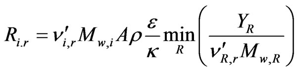 (14)
(14)
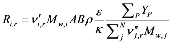 (15)
(15)
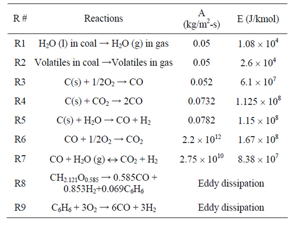
Table 1. Global gasification reactions model (n = 0).
whereYP is the mass fraction of any product species P;
YR is the mass fraction of a particular reactant R;
A is an empirical constant equal to 4.0;
B is an empirical constant equal to 0.5;
 is the stoichiometric coefficient for reactant i in reaction r;
 is the stoichiometric coefficient for product j in reaction r;
Mw,i, Mw,j, and Mw,R are the molecular weight of species i, j and a particular reactant R, respectively.
The Finite-Rate Model computes the chemical source terms using Arrhenius expressions and ignores the effects of turbulent fluctuations. The net source of chemical species i due to reaction Ri (kg/m3-s) is computed as the sum of the Arrhenius reaction sources over the NR reactions that the species participate in, and is given as:
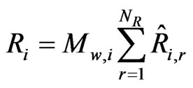 (16)
(16)
where  is the Arrhenius molar rate of production/ consumption of species i in reaction r.
The r-th reaction can be written in a general form as:
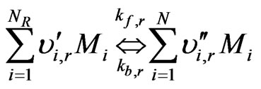 (17)
(17)
where kf,r = forward rate constant for reaction r;
kb,r = backward rate constant for reaction r.
The molar reaction of production/consumption of species i as a result of reaction r, which is  (kmol/m3-s) in Equation (16), is given as:
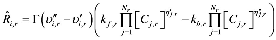 (18)
(18)
whereCj,r = molar concentration of each reactant and product species j in reaction r (kmol/m3);
 = forward rate exponent for each reactant and product species j in reaction r;
 = backward rate exponent for each reactant and product species j in reaction r.
For Heterogeneous Reactions, the particle reaction, R (kg/m2-s), is expressed as:
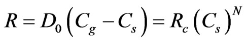 (19)
(19)
where D0 = bulk diffusion coefficient (m/s);
Cg = mean reacting gas species concentration in bulk (kg/m³);
Cs = mean reacting gas species conc. at particle surface (kg/m²);
Rc = chemical reaction rate coefficient (units vary);
N = apparent reaction order (dimensionless).
The concentration at the particle surface, Cs, is not known, so it is replaced by other quantities, and the expression is recast as follows:
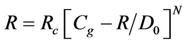 (20)
(20)
This equation has to be solved by an iterative procedure, with the exception of the cases when N = 1 or N = 0. When N = 1, Equation (20) can be written as
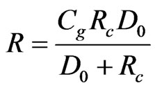 (21)
(21)
The reaction stoichiometry of a particle undergoing an exothermic reaction in a gas phase is given as:
particle species j (s) + gas phase species n ® products.
Its reaction rate is given as:
 (22)
(22)
where
 (23)
(23)
and where the quantities
 = rate of particle surface species depletion (kg/s);
Ap = particle surface area (m2);
Yj = species fraction;
hr = effectiveness factor (dimensionless);
 = rate of particle surface species reaction per unit area (kg/m2-s);
pn = bulk concentration of the gas phase species (kg/m3);
D0,r = diffusion rate coefficient for reaction r;
Rkin,r = kinetic rate of reaction r (units vary), and;
Nr = apparent order of reaction r.
The effectiveness factor, r, is related to the surface area, and can be used in each reaction in the case of multiple reactions.
D0,r is given by
 (24)
(24)
Equation (24) is a modification of the relationship given by Smith [35] by assuming negligible change in gas density.
The kinetic rate of reaction r is defined as
 (25)
(25)
The rate of particle surface species depletion for reaction order Nr = 1 is given by:
 (26)
(26)
And for reaction order Nr = 0, the rate of depletion is given by:
 (27)
(27)
5. Computational Scheme
5.1. Computational Grid
The geometry is generated and meshed in GAMBIT Version 2.4.6, using a 2-D grid (Figure 5). Structured grids are used in the draft tube and syngas exit areas and unstructured grids are used in rest of the areas. For this preliminary study, a total of 30,876 cells are employed. The y+ values of the first near-boundary grid point vary between 20 and 50 in the draft tube and are between 50 and 150 in the fluidized bed and freeboard regions. y+ is a modified distance from wall and defined as y+ = ρv*y/µ, where v* is the frictional velocity and defined as  and τW is the wall shear stress. The enhancedwall function will automatically fill in the near-wall turbulence structure below the first near-wall grid points.
5.2. Boundary and Inlet Conditions
The following boundary conditions on the surface geometry have been assigned.
1) Velocity inlet: At all the inlet surfaces, the velocity, temperature, and the mass fractions of all species of the gas mixture are specified in Table 2.
2) Pressure outlet: The outlet surface is assigned as a constant pressure boundary. In this study, flow separation occurs at the gas exit due to the sharp 90-degree connection of the external ducts. For flow separation, the backflow condition needs to be specified. Typically, a preliminary study is conducted, and the result of the flow
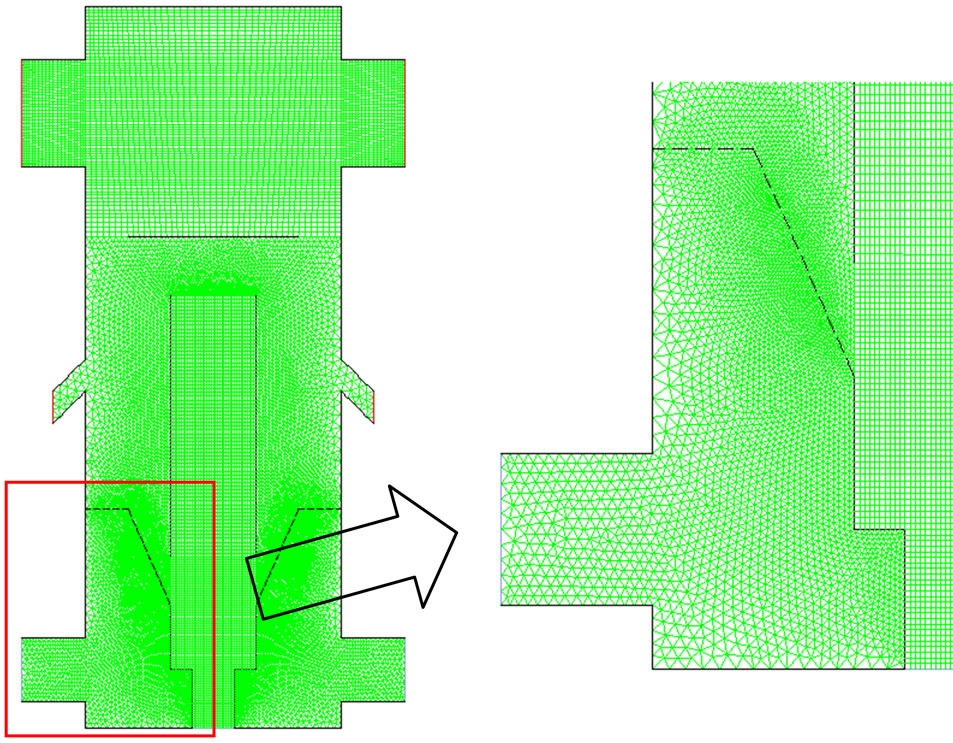
Figure 5. Mesh for the computational domain.
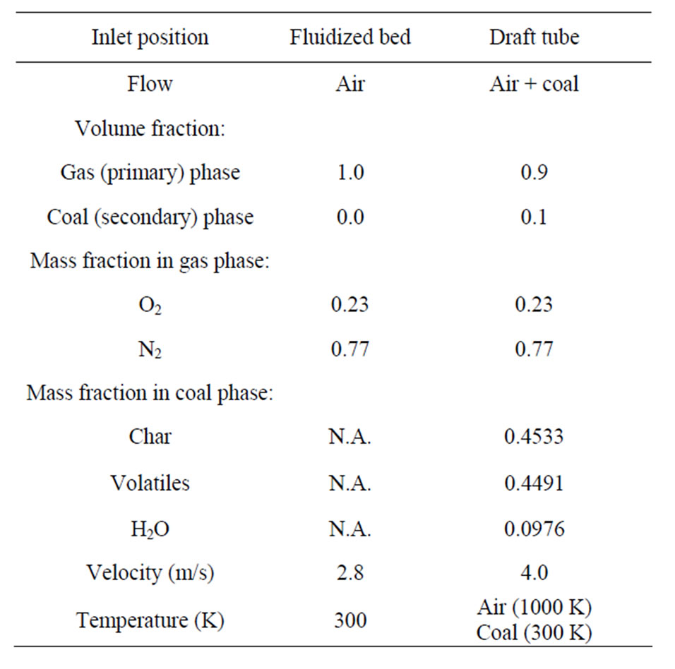
Table 2. Flow condition at inlets of the fluidized bed and draft tube.
condition and species composition at the exit are assigned as the backflow’s condition. Several iterations will be taken until the results converge. However, it is found during the preliminary study that assignment of syngas composition in the backflow makes reporting freshly produced syngas composition unclear because the backflow syngas contaminates the calculation of syngas composition at the exit. This issue is exacerbated by the transient simulation conducted in this study because the exit flow condition continuously changes at each new instant. To resolve this issue, the backflow is intentionally assigned without containing any syngas so the mass flow weighted calculation of the syngas at the exit consists entirely of the freshly produced syngas. This approach would only limitedly affect the diffusion terms near the exit without affecting the results inside the gasifer.
3) Walls: The outside surfaces are defined as a wall boundary. The walls are stationary with the no-slip condition imposed (zero velocity) on the surface and are assumed to be well insulated with zero heat flux (i.e., the adiabatic condition).
4) Fluidized bed: The bed is initially filled with char (C) with a depth of 10 inches. The char outlets are designed to allow controlling of the bed depth by valves. In the CFD simulation, the char extracting rate is controlled by changing the char outlets’ pressure values. This is done by initially filling the bed with coal (100% solid carbon + 0% H2O vapor + 0% volatiles) with 40% void.
5) Patching temperature: Akin to using a lighter to ignite combustion inside a combustor, a high temperature is needed to start (ignite) the reactions by setting the initial temperature of the cells near the injectors to 1000 K.
5.3. Numerical Procedure
The commercial CFD software package, ANSYS/FLUENT 12.0, was used in this study. The governing equations are discretized spatially with second-order accuracy to yield discrete algebraic equations for each control volume. The volume fraction of the solid phase is calculated using the QUICK scheme. The SIMPLE algorithm [36] is used in this study to couple the pressure and velocity.
The primary phase (gas) enters the computational domain through the inlets. The iterations are conducted alternatively between the primary phase and the secondary phase (coal). The primary phase is updated in the next iteration based on the secondary phase calculation results, and the process is repeated. Unsteady flow calculations are performed.
The computations are conducted via two clusters with 8 dual-core personal computers on each cluster. The physical iteration time step size is chosen to be 10−4 seconds. Typically, 6000 time steps (up to 0.6 seconds, more than twice the residence time of coal from inlet to outlet) are required in two calendar days to achieve convergence with 250 iterations (at best) in each time step. However, the studied case is run with 24,000 time steps up to 2.4 seconds.
Since there is no experimental data available for comparison, implementation of the model starts from simulating single-phase turbulent flow and heat transfer to understand the thermal-flow behavior, followed by employing demoisturization, devolatilization and seven global gasification and thermal cracking reactions, progressively adding one equation at a time. Finally, the particles are introduced. The detailed description of the development and qualification of the reactive multiphase CFD model was documented by Mazumder and Wang [24] and Monayem et al. [25,26].
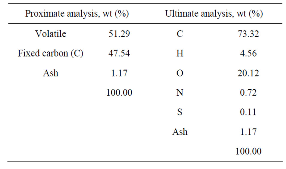
The coal used in this study is an Indonesian coal. The proximate and ultimate analyses are given below:
6. Results and Discussions
6.1. Devolatilization
The main objective of this study is to implement a demoisturization and devolatilization model and implement it in the existing commercial code. Since there is no experimental data available for verification, the successful implementation of the demoisturization and devolatilization mechanisms is judged by cross-examining the reduction of the water and volatiles mass-fraction changes in the coal phase and the concurrent generation of water and volatiles in the gas phase as demonstrated in Figures 6 and 7. Figure 6 shows snapshots of the dynamic evolution of the mass fraction of volatiles in the coal phase in a 0.5 sec time step up to 2 seconds. The coal is seen to progressively lose volatiles throughout the draft tube. No notable devolatilization occurs in the fluidized bed area until after 1 sec. Approximately 25% of the volatiles remain in the coal at the syngas exits at the end of 2 sec.
Loss of water and volatiles in coal should appear in the gas phase. Indeed this complementary phenomenon is seen as the mass fractions of water vapor and volatiles progressively increase with time in Figures 7 and 8. This is the first indication of successful implementation of the demoisturization and devolatilization process in the computational code. The ongoing demoisturization and devolatilzation process can be also observed by the increased coal density shown in Figure 9 because the densities of volatiles and moisture are lighter than the char.
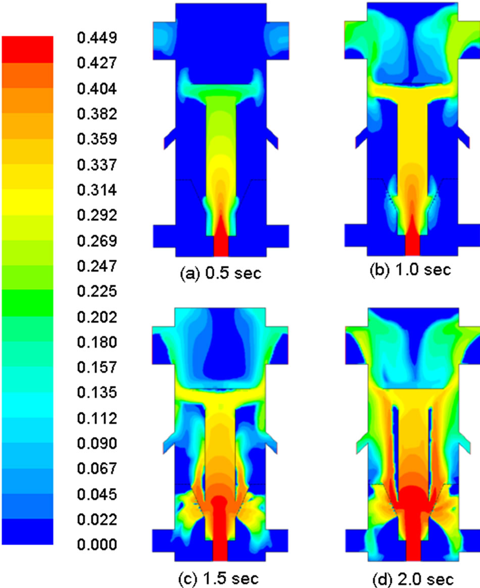
Figure 6. Distribution of mass fraction of volatiles in coal in different times.
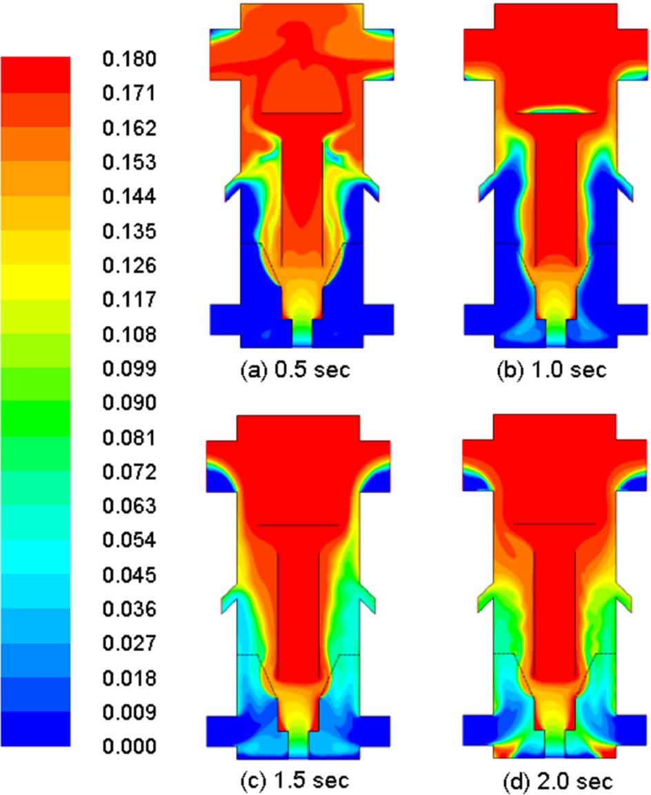
Figure 7. Distribution of mass fraction of moisture in gas in different times.
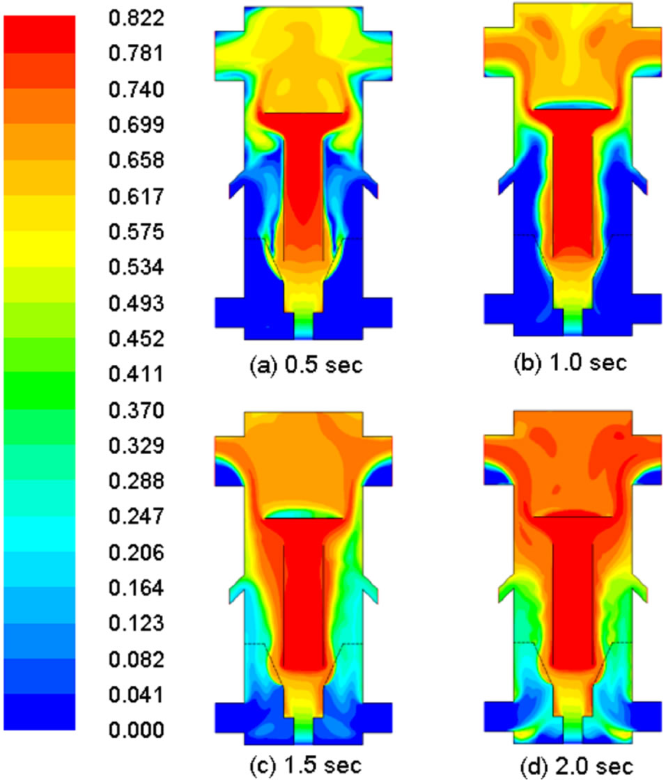
Figure 8. Distribution of mass fraction of volatiles in gas in different times.
6.2. Flow Behavior
Figure 10 shows snapshots of the dynamic change of coal
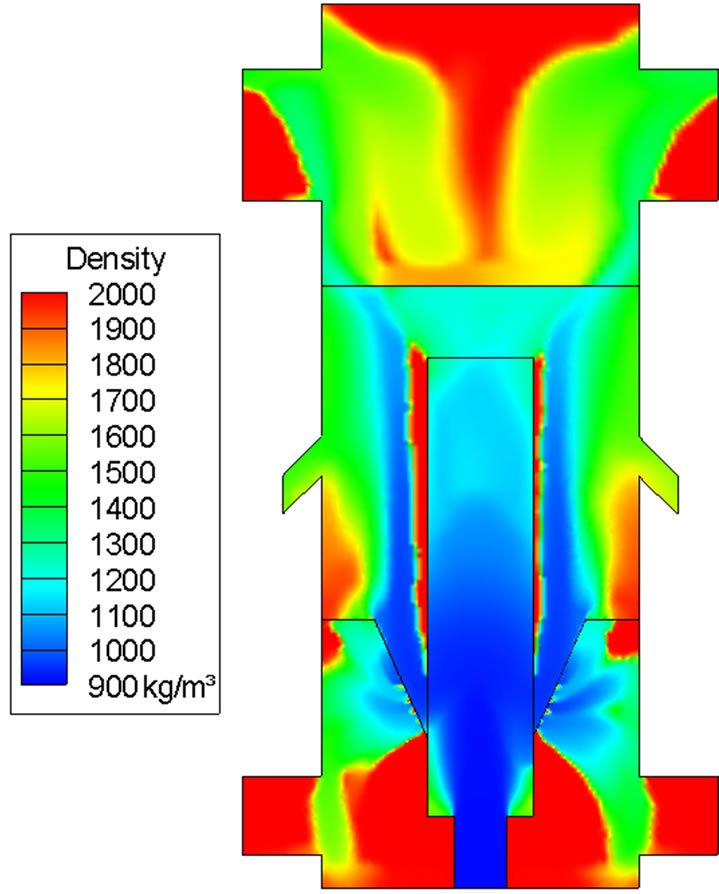
Figure 9. Coal density distribution at 2 sec. The pure char density is 2000 kg/m3. Note that high coal density area does not necessarily mean high coal mass fraction. It only means that the coal in that area is close to the property of char.
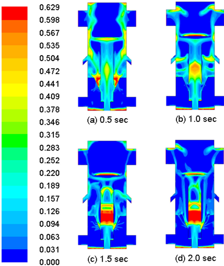
Figure 10. Distribution of coal volume fraction in different times.
volume fraction in each 0.5 sec time step. It needs to be noted that the actual process can be better seen and understood in an animated movie, which can’t be shown in this paper, but is used to help explain the flow physics and phenomenon below. The animated movie shows that the flow does not reach “steady state”, rather it reaches “periodic steady state” at about 2 seconds. The period of each cycle is about 0.5 seconds. The periodicity is demonstrated both inside the draft tube and in the fluidized bed area. Inside the draft tube, the coal seems accumulated and choked half way through, as can be seen from the red high-density regions in Figures 10(c) and (d). This highdensity region is seen to be stationary, but periodic highdensity patches are ejected upward alternately from this accumulated region. Figure 10(c) at 1.5 sec happens to capture a new patch just leaving the accumulated area and a previous batch already traveling to the draft tube exit. Figure 10(d) at 2 sec shows another new patch has been ejected.
It is interesting to note that a layer of char accumulates on top of the deflector. This layer is formed from deposition of char dust falling from upper chamber of the gasifier. To reduce char accumulation, the deflector can be designed in the shape of a dome to allow this char dust to slide down.
In the fluidized bed area, the periodic flow pattern is manifested as a large coherent structure in the form of alternating, up-swelling puffs and granular flow circulations. Just examining the evolution of the mole-fraction of char is not sufficient to obtain an overall picture of the multiphase flow motions, especially since the gases and solids can move in different ways. Therefore, Figures 11 and 12 are provided by showing the velocity fields of the gas and solid phases separately. Figure 11 shows the gas velocity reaches periodic steady state after 1.5 sec. The flow in the fluidized bed region and draft tube are all moving upward. A wake region formed as a closed separation bubble appears behind (on top of) the deflector at 0.5 s in Figure 11(a), but the wake region disappears later in Figure 11(b). As the gas phase moves upward in the fluidized bed, the coal particle phase is actually moving downward as shown in Figure 12(a) at 0.5 sec. Some of the coal particles are shown being entrained into the draft tube from the fluidized bed in Figure 12(a), while no gases seem to be entrained in a similar way in Figure 11.
It is important to note that since the multiphase flows are periodic, the transient computational method and associated transient governing equations must be used to adequately capture the periodic activities. The patterns of all the figures are symmetric, indicating good-quality computation has been achieved for this complex reactive multiphase flow.
6.3. Mild Gasification
The goal for mild gasification can be achieved if volatiles can be collected as high-energy fuels that have not yet been consumed by combustion or thermally cracked to lighter gases like CO and H2. Figure 13 shows that a large portion of volatiles is successfully preserved under the simulated operating condition, which is encouraging for moving forward to conduct further parametric studies and build the test model.
Figure 13 shows the temperature distribution of gas and coal. The gas phase temperature is 367.1 K (200˚F)
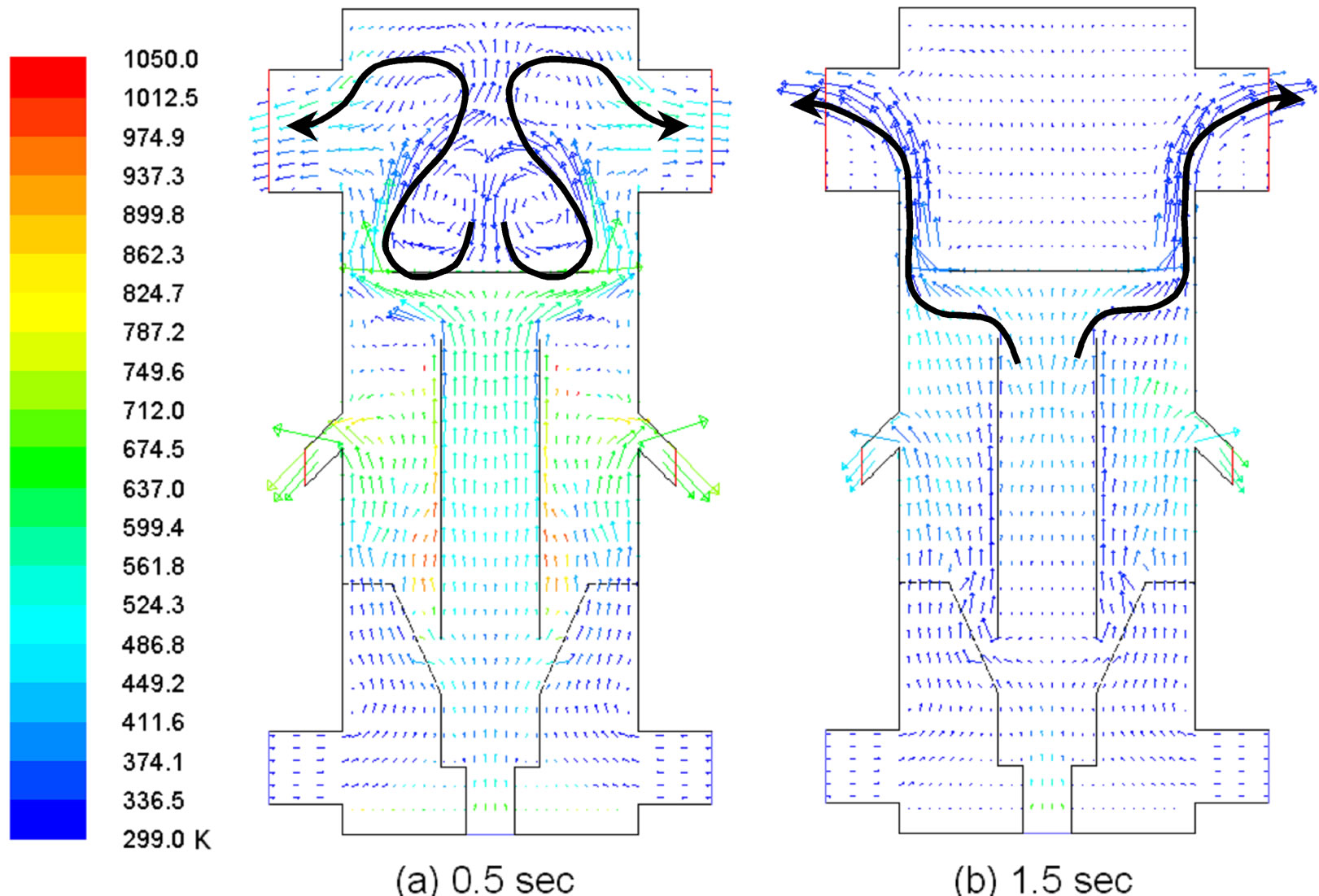
Figure 11. Gas flow field showing large circulations close to the exit at 0.5 and 1.5 sec.
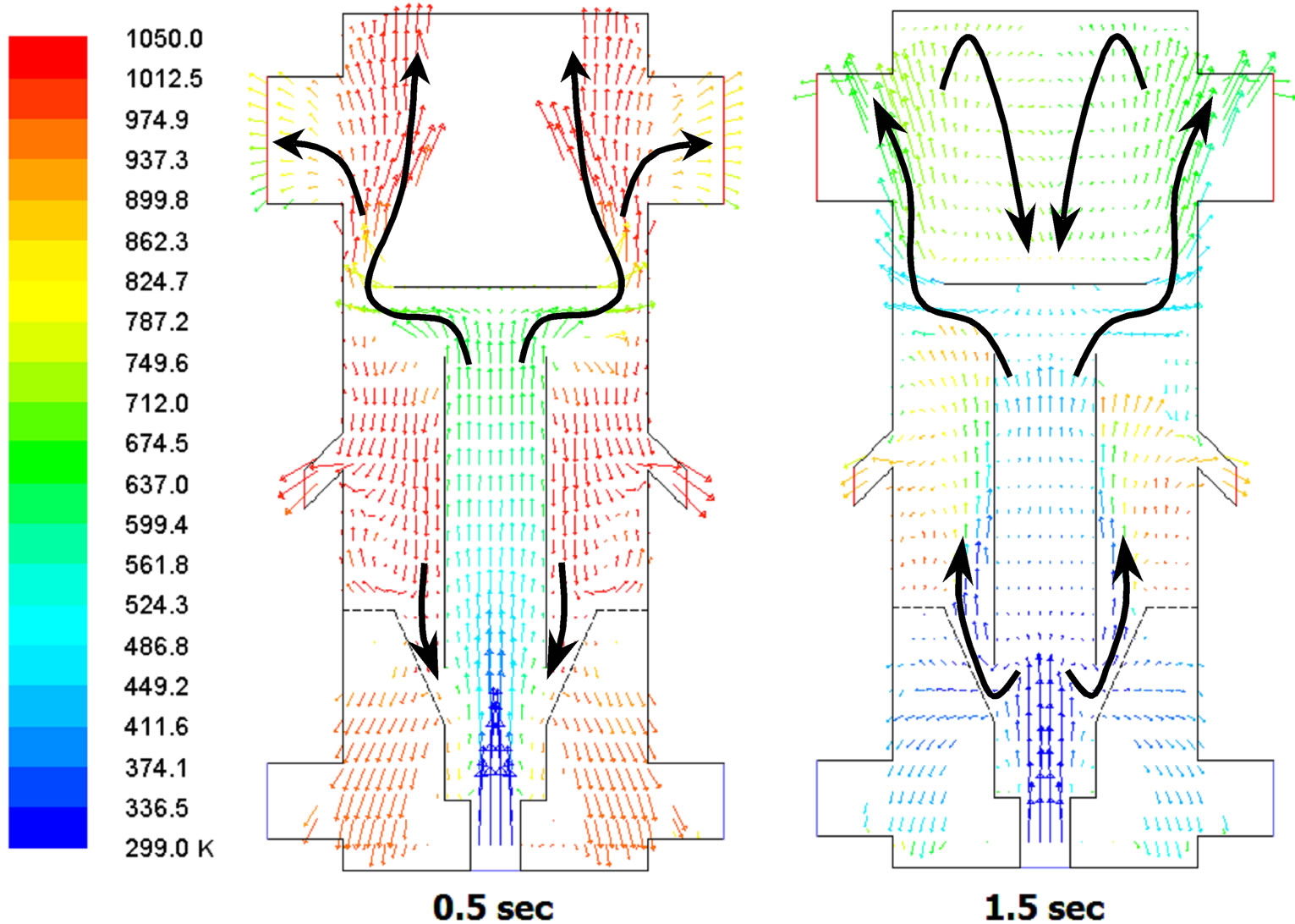
Figure 12. Coal particle velocity colored by coal temperature (entrainment shown with arrow) at 0.5 sec and 1.5 sec.
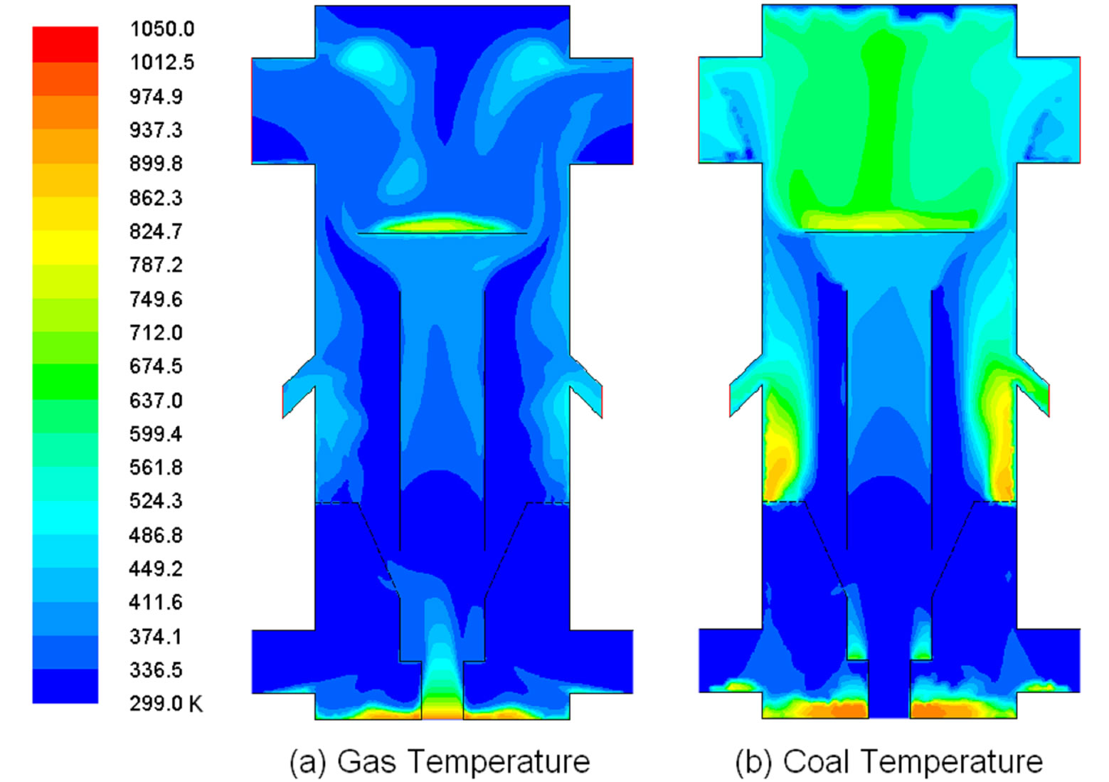
Figure 13. Distribution of gas and coal temperature at 2 sec.
at the syngas outlet and 426.1 K (307˚F) at the char chute outlet. This temperature difference implies that some endothermic gasification reactions (R3 and R4) occur in the upper part of the gasifier, as can be evidenced from the progressively increased productions of H2 and CO between the exit of draft tube and the syngas outlet in Figure 13. On the other hand, the coal phase exit temperatures are 490.2 K (422˚F) at syngas outlet and 600.9 K (621˚F) at char outlet. The solid phase is about 120 K (216˚F) hotter than the syngas at the syngas outlet and 160 K (288˚F) hotter at the char outlet. The hottest gas temperature is about 975 K (1286˚F) at the draft tube inlet and the hottest coal temperature is about 900 K (1160˚F) in the fluidized bed and on top of the deflector. These temperatures are significantly lower than a full-gasification gasifier, indicating less energy is used in mild gasification.
Table 3 provides more detailed data of syngas composition at the syngas outlet, which consists of 70.88% (wt) volatiles (64.87% vol) 6.01% wt (4.55% vol) CO, and 0.63% wt (6.63% vol) H2. Both H2 and CO are desired products for a full gasification process, but, in this study, lower amounts of H2 and CO is another indicator confirming that mild-gasification is successfully achieved.
The syngas also contains an appreciable amount of unreacted char dust (78% wt, 15.03% vol), which can be collected and recycled to the gasifier or boiler through cyclones (see Figure 2). The carbon conversion rate is 0.017%, the devolatilization rate is 60.17%, and the high heating value (HHV) of the syngas is 16.64 MJ/kg, which is about 1/3 of natural gas’s HHV.
The desired mild-gasifier design intends to produce “clean coal” (or pure char) and transport it to the traditional pulverized coal (PC) boiler through the char chutes. This is why the carbon conversion rate is very low in this study. Table 4 provides the material composition of the produced char at the exit of the char chutes, showing 78.97% (wt) solid carbon, 17.29% (wt) volatiles, and 3.75% (wt) moisture. However, very little char (only 1.72% in volume) is present at the char chutes, as shown in Figure 14. This is not ideal. A further investigation by examining the CFD animation discovered that the fluidized bed can’t be maintained at the same height becausemore char is drained out from the char chute and/or carried away by syngas than is provided at the inlet. At about 0.16 sec, the fluidized level becomes lower than
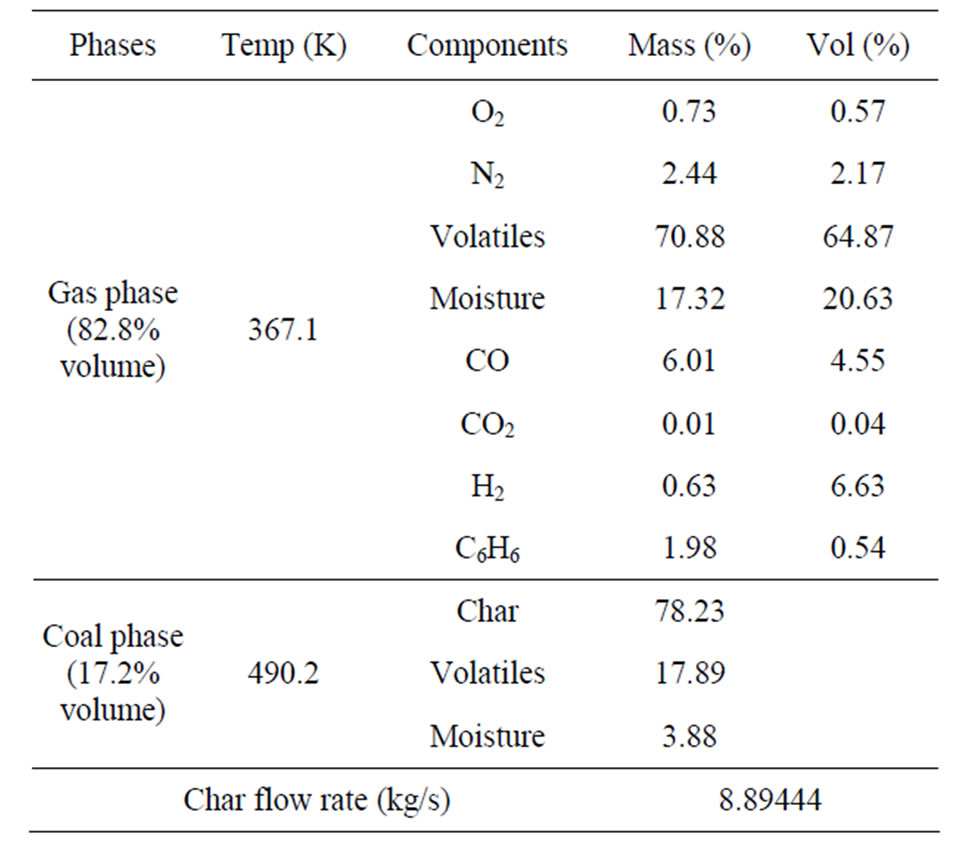
Table 3. Multiphase material composition at the syngas outlet at 2 sec.
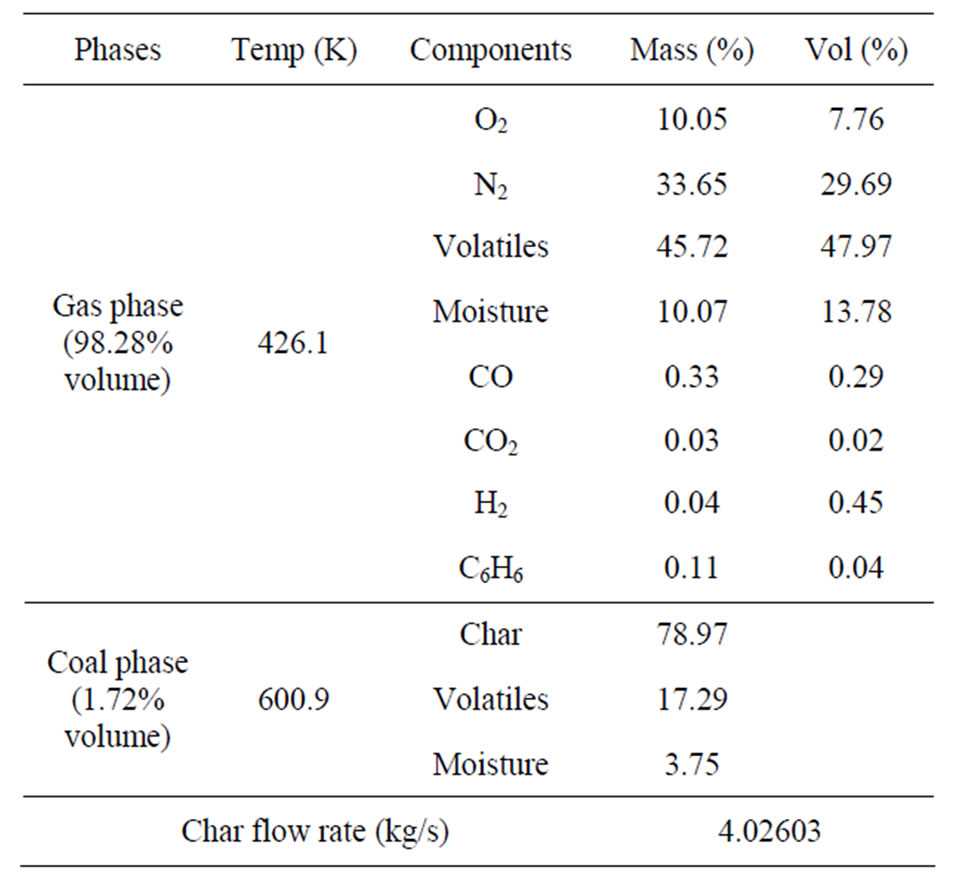
Table 4. Multiphase material composition at the inlet to char chute at 2 sec.
the char chute and continuous fluidization can’t be maintained against 1.5 m/s fluidization air velocity because of the shallow bed’s light weight, so the remaining char in the bed was blown away by the fluidization air. Figure 15 shows the history of the changing fluidized bed height and coal volume fraction at the char chute exits. This figure shows that the char chute extracts the maximum amount of char at 0.16 sec and the entire bed is blown away after 0.24 sec.
This result, although not ideal, is very intriguing and useful and has led to the following revisions of gasifier design and operating conditions:
1) In the real operation, the char extraction rate can be controlled by a valve to reduce the char extraction rate. In the CFD simulation, this can be done by reducing the diameter of the char chute or increase the pressure at char chute’s exit.
2) To keep the weight of the bed sufficient for fluidization, the location of the char chutes can be raised higher. In the meantime, the fluidization velocity can be also reduced simultaneously.
3) A large amount of char has been carried away with the syngas; the carried-away char loss can be minimized by reducing the draft tube inlet velocity as well as the fluidization velocity.
7. Conclusions
The results are summarized below:
1) The devolatilization model (including the demoisturization process) has been successfully implemented in the computational code, ANSYS/FLUENT. This model needs to be calibrated by experimental data in the future.
2) A large amount of volatiles are successfully pre-
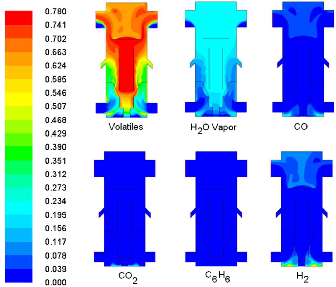
Figure 14. Volumetric fraction of major gases at 2 sec.
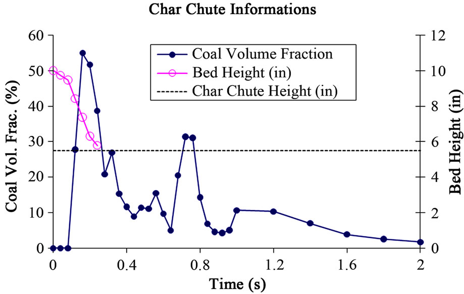
Figure 15. The history of fluidized bed height and coal volume fraction extracted at the exit of char chutes.
served as a high-energy fuel in the syngas stream.
3) The conceptual design of the mild gasifier test model is promising and the CFD result shows that the desired degree of mild gasification can be achieved.
4) The deflector is found effective in deflecting the majority of coal particles, but its configuration needs to be redesigned as a dome shape to minimize deposition of coal particles on its roof.
5) An appreciable amount (78% wt) of char is carried away by the syngas stream to the exit. The gas flow velocity in the draft tube as well as in the fluidized bed can be turned down to reduce char escape rate.
6) The fluidized bed is not sustainable under the present operating condition. This can be resolved by reducing the char chute diameter, raising the char chute higher, and/or reducing the fluidization velocity.
The results of this study are very encouraging. The mild gasification is achieved partially under the simulated operating conditions. It seems achieving a different degree of mild-gasification process can be effectively controlled by changing the operating conditions such as oxygen amount, operating pressure, fluidization gas flow rate, the char entrainment rate from the fluidized bed to the draft tube, replacing fluidization air with recycled raw syngas, etc. The CFD model, implemented with the newly developed devolatilization model, is shown to be a very valuable and effective tool to help guide design of the mild gasifier test model and associated operating conditions to achieve various degrees of mild gasification.
8. Acknowledgements
This study was partially supported by the Louisiana Governor’s Energy Initiative via the Clean Power and Energy Research Consortium (CPERC) under the auspices of Louisiana Board of Regents and partially supported by the Department of Energy contract NO. DEFC26-08NT01922.
REFERENCES
- D. B. Anthony, J. B. Howard, H. C. Hottel and H. P. Meissner, “Rapid Devolatilization of Pulverized Coal,” 15th International Symposium on Combustion, Tokyo, 25-31 August 1975, pp. 1303-1317.
- S. Ergun, “Fluid Flow through Packed Columns,” Journal of Chemical Engineering Progress, Vol. 48, No. 2, 1952, pp. 89-94.
- M. Syamlal and D. Gidaspow, “Hydrodynamic of Fluidization: Prediction of Wall to Bed Heat Transfer Coefficients,” AIChE Journal, Vol. 31, No. 1, 1985, pp. 127- 135. doi:10.1002/aic.690310115
- M. Syamlal, “The Particle-Particle Drag Term in a MultiParticle Model of Fluidization,” Topical Report, Work Performed under Contract No.: DE-AC21-85MC21353, 1987.
- W. C. Yang and D. L. Keairns, “Rate of Particle Separation in a Gas Fluidized Bed,” Journal of Industrial Engineering Chemical Fundamentals, Vol. 21, No. 3, 1982, pp. 228-235. doi:10.1021/i100007a007
- M. Syamlal and T. J. O’Brien, “Computer Simulation of Bubbles in a Fluidized Bed,” AlChE Symposium Series, Vol. 85, No. 270, 1989, pp. 22-31.
- D. J. Gunn, “Transfer of Heat or Mass to Particles in Fixed and Fluidized Beds,” Journal of Heat Mass Transfer, Vol. 21, No. 4, 1978, pp. 467-476. doi:10.1016/0017-9310(78)90080-7
- C. K. K. Lun, S. B. Savage, D. J. Jeffrey and N. Chepurniy, “Kinetic Theories for Granular Flow: Inelastic Particles in Couette Flow and Slightly Inelastic Particles in a General Flowfield,” Journal of Fluid Mechanics, Vol. 140, 1984, pp. 223-2565. doi:10.1017/S0022112084000586
- S. B. Savage and D. J. Jeffrey, “The Stress in a Granular Flow at High Shear Rates,” Journal of Fluid Mechanics, Vol. 110, 1981, pp. 255-272. doi:10.1017/S0022112081000736
- J. A. M. Kuipers, W. Prins and W. P. M. Van Swaaij, “Numerical Calculation of Wall-to-Bed Heat-Transfer Coefficients in Gas-Fluidized Beds,” AlChE Journal, Vol. 38, No. 7, 1992, pp. 1079-1091. doi:10.1002/aic.690380711
- H. Enwald and A. E. Almstedt, “Fluid Dynamics of a Pressurized Fluidized Bed: Comparison between Numerical Solutions from Two-Fluid Models and Experimental Results,” Journal of Chemical Engineering Science, Vol. 54, No. 3, 1999, pp. 329-342. doi:10.1016/S0009-2509(98)00187-0
- V. Jiradilok, D. Gidaspow, S. Damronglerd, W. J. Koves and R. Mostofi, “Kinetic Theory Based CFD Simulation of Turbulent Fluidization of FCC Particles in a Riser,” Chemical Engineering Science, Vol. 61, No. 17, 2006, pp. 5544-5559. doi:10.1016/j.ces.2006.04.006
- R. Panneerselvam, S. Savithri and G. D. Surneder, “CFD Based Investigation on Hydrodynamics and Energy Dissipation Due to Solid Motion in Liquid Fluidized Bed,” Journal of Chemical Engineering, Vol. 132, No. 1-3, 2007, pp. 159-171. doi:10.1016/j.cej.2007.01.042
- N. Reuge, L. Cadoret, C. C. Saudejaud, S. Pannala, M. Syamlal and B. Caussat, “Multifluid Eulerian Modeling of Dense Gas-Solid Fluidized Bed Hydrodynamics: Influence of the Dissipation Parameters,” Journal of Chemical Engineering Science, Vol. 63, No. 22, 2008, pp. 5540- 5551. doi:10.1016/j.ces.2008.07.028
- Department of Energy, National Energy Technology Laboratory, “Multiphase Flow with Interphase eXchange,” 2012. https://mfix.netl.doe.gov/
- F. Chejne and J. P. Hernandez, “Modeling and Simulation of Coal Gasification process in Fluidized Bed,” Fuel, Vol. 81, No. 13, 2002, pp. 1687-1702. doi:10.1016/S0016-2361(02)00036-4
- L. Yu, J. Lu, X. Zhang and S. Zhang, “Numerical Simulation of the Bubbling Fluidized Bed Coal Gasification by the Kinetic Theory of Granular Flow (KTGF),” Fuel, Vol. 86, No. 5-6, 2007, pp. 722-734. doi:10.1016/j.fuel.2006.09.008
- X. Wang, B. Jin and W. Zhong, “Three-Dimensional Simulation of Fluidized Bed Coal Gasification,” Chemical Engineering and Processing: Process Intensification, Vol. 48, No. 2, 2009, pp. 695-705. doi:10.1016/j.cep.2008.08.006
- A. Suo-Anttila, J. D. Smith and L. D. Berg, “Development and Application of an LES Based CFD Code to Simulate Coal and Biomass Combustion in General Reactor Configurations,” 9th European Conference on Industrial Furnaces and Boilers, Estoril, 26-29 April 2011.
- R. Gupta, B. Turk and M. Lesemann, “RTI/Eastman Warm Syngas Clean-Up Technology: Integration with Carbon Capture,” Presented at the 2009 Gasification Technologies Conference, 2009.
- R. Gupta, A. Jamal, B. Turk and M. Lesemann, “Scaled and Commercialization of Warm Syngas Cleanup Technology with Carbon Capture and Storage,” Presented at the 2010 Gasification Technologies Conference, Washington DC, 2010.
- A. Wormser, “Repowering Steam Plants with Mild Gasification IGCCs,” Proceedings of the 24th International Pittsburgh Coal Conference, Johannesburg, 10-14 September 2007.
- A. Wormser, “Converting PC to Very-High-Efficiency IGCC: The MaGICTM of Mild Gasification,” Modern Power System, November 2008, pp. 21-26.
- A. K. M. Mazumder and T. Wang, “Development of a Simulation Model for Fluidized Bed Mild Gasifier,” ECCC Report 2010-05, Energy Conversion and Conservation Center, University of New Orleans, November 2010.
- A. K. M. Mazumder, T. Wang and J. R. Khan, “Design and Simulation of a Mild Gasifier, Part 1—Development of a Multiphase Computational Model,” ASME Paper IMECE 2011-64473, Proceedings of the ASME International Mechanical Engineering Congress & Exposition, Denver, 11-17 November 2011.
- A. K. M. Mazumder, T. Wang and J. R. Khan, “Design and Simulation of a Mild Gasifier, Part 2—Case Study and Analysis,” ASME Paper IMECE 2011-64485, Proceedings of the ASME International Mechanical Engineering Congress & Exposition, Denver, 11-17 November 2011.
- H. Kobayashi, J. B. Howard and A. F. Sarofim, “Coal Devolatilization at High Temperatures,” 16th Symposium (International) on Combustion, The Combustion Institute, 1976.
- S. Badzioch and P. G. W. Hawsley, “Kinetics of Thermal Decomposition of Pulverized Coal Particles,” Industrial & Engineering Chemistry Process Design and Development, Vol. 9, No. 4, 1970, pp. 521-530. doi:10.1021/i260036a005
- M. M. Baum and P. J. Street, “Predicting the Combustion Behavior of Coal Particles,” Combustion Science and Technology, Vol. 3, 1971, pp. 231-243.
- K. K. Pillai, “The Influence of Coal Type on Devolatilization and Combustion in Fluidized Beds,” Journal of the Energy Institute, Vol. 54, 1981, pp. 142-150.
- T. H. Fletcher, A. R. Kerstein, R. J. Pugmire and D. M. Grant, “Chemical Percolation Model for Devolatilization: 2. Temperature and Heating Rate Effects on Product Yields,” Energy Fuels, Vol. 4, No. 1, 1990, pp. 54-60. doi:10.1021/ef00019a010
- T. H. Fletcher and A. R. Kerstein, “Chemical Percolation Model for Devolatilization: 3. Direct Use of CNMR Date to Predict Effects of Coal Type,” Energy Fuels, Vol. 6, No. 4, 1992, pp. 414-431. doi:10.1021/ef00034a011
- D. M. Grant, R. J. Pugmire, T. H. Fletcher and A. R. Kerstein, “Chemical Percolation of Coal Devolatilization Using Percolation Lattice Statistics,” Energy Fuels, Vol. 3, No. 2, 1989, pp. 175-186. doi:10.1021/ef00014a011
- A. Silaen and T. Wang, “Effect of Turbulence and Devolatilization Models on Coal Gasification Simulation in an Entrained-Flow Gasifier,” International Journal of Heat and Mass Transfer, Vol. 53, No. 9-10, 2010, pp. 2074- 2091. doi:10.1016/j.ijheatmasstransfer.2009.12.047
- I. W. Smith, “The Combustion Rates of Coal Chars: A Review,” 19th International Symposium on Combustion, Vol. 19, No. 1, 1982, pp. 1045-1065.
- S. V. Patankar, “Numerical Heat Transfer and Fluid Flow,” McGraw Hill, New York, 1980.