International Journal of Modern Nonlinear Theory and Application
Vol.3 No.2(2014), Article
ID:46902,7
pages
DOI:10.4236/ijmnta.2014.32006
A Method for Finding Optimal Parameter Values Using Bifurcation-Based Procedure
Hiroyuki Kitajima1, Tetsuya Yoshinaga2
1Faculty of Engineering, Kagawa University, Takamatsu, Japan
2School of Health Sciences, Tokushima University, Tokushima, Japan
Email: kitaji@eng.kagawa-u.ac.jp, yosinaga@medsci.tokushima-u.ac.jp
Copyright © 2014 by authors and Scientific Research Publishing Inc.
This work is licensed under the Creative Commons Attribution International License (CC BY).
http://creativecommons.org/licenses/by/4.0/


Received 3 May 2014; revised 3 June 2014; accepted 9 June 2014
Abstract
In dynamical systems, the system suddenly becomes unstable due to parameter perturbation which corresponds to environmental changes or major incidents. To avoid such instabilities in engineering systems, tuning system parameters is very important. In this paper, we propose a method for obtaining optimal parameter values in a parameterized dynamical system. Here, the optimal value means the farthest point from the bifurcation curves in a bounded parameter plane. As illustrated examples, we show the results of continuous-time and discrete-time systems. Our algorithm can find the optimal parameter values in both systems.
Keywords
Bifurcation, Stability, Dynamical System

1. Introduction
The aim of our study is to construct a system that is robust to sudden environmental changes and major incidents. Such changes trigger instabilities in the system, called bifurcations. In biological systems, for example, dynamical diseases such as Cheyne-Stokes respiration and chronic granulocytic leukemia are caused by bifurcations due to variations in system parameters [1] [2] . The ability to predict bifurcations in a parameter space is very important to preventing such diseases. Several methods of predicting and controlling bifurcations have proposed such as, using the averaged harmonic method [3] , constructing a feedback system [4] -[6] , and minimizing the maximum eigenvalues of symmetric matrices through optimization [7] -[9] . The methods in cited studies aim to minimize the maximum eigenvalues of the linearized system (Jacobian matrix), which correspond to rapid recovery from a perturbed state.
However, a parameter value with a minimum eigenvalue does not have the longest margin to bifurcations in the parameter space. Dobson proposed a method of calculating the closest-bifurcation from the operating parameter values [10] . This method and its extensions have been applied to hydraulic systems [11] , gene systems [12] , power systems [13] [14] , and bifurcations of arbitrary codimension [15] . Moreover, another method using support vector machine (SVM) and particle swarm optimization (PSO) was proposed [16] . However, in all of the above cases, the considered bifurcations are only for equilibrium points.
In this paper, we propose a method to calculate the closest-bifurcation for periodic solutions by constructing vector fields along bifurcation curves. Moreover, we extend the notion of the closest-bifurcation in order to search for the optimal parameter value, which means the farthest point from the bifurcations in the parameter region under consideration. As a result, we can set appropriate parameter values that correspond to constructing a system which is robust to unexpected parameter changes.
2. Method
2.1. Dynamical System
We consider the following autonomous dynamical system:
 (1)
(1)
where  is a controllable parameter and
  is a state variable. We assume that there exists a periodic solution in Equation (1) with an initial condition
  at
at , denoted by
  for all t. We take a local section
 , that the solution crosses transversely, as follows:
 (2)
(2)
where  is a scalar valued function of
  in
in . Let us define h as a local coordinate of
 (3)
(3)
and its inverse  as an embedding map
 (4)
(4)
where  satisfies
 . Pick a point
  and let
  be some neighborhood of
 . Then the Poincaré map T is defined by the following composite map for a point
 :
:
 (5)
(5)
where  denotes the time during which the trajectory emanating from a point
  hits the local cross-section
  again. The time
  is called the return time.
Similarly, for a non-autonomous system,
 (6)
(6)
we can construct the Poincaré map T as
 (7)
(7)
where L is the period of the function :
:
 (8)
(8)
For a discrete system, the map T is directly obtained by
 (9)
(9)
For all dynamical systems, the fixed point of the map T is given by
 (10)
(10)
In the differential equations, we can obtain a one-to-one correspondence between the periodic solution of Equation (1) or Equation (6) and the fixed point of the map T. Hence, the analysis of the periodic solution can be reduced to an analysis of the fixed point of the map T. The characteristic multiplier  of the fixed point
  is obtained by solving
 (11)
(11)
where
 (12)
(12)
If all absolute values of the characteristic multipliers are less than one, then the fixed point is stable. The change in stability due to a parameter perturbation is called a bifurcation. The codimension-one bifurcations are as follows: when ,
,  and
and , the tangent, period-doubling, and NeimarkSacker bifurcations occur, respectively.
2.2. Search for Optimal Parameter Values
Here, we describe our method of searching for the optimal parameter values that are farthest points from bifurcations in the parameter region under consideration. For this, we extend the idea of the closest-bifurcation method proposed by Dobson [10] . This method determines the minimum distance to bifurcations along selected directions in the parameter space. It searches a local region of the parameter space in order to find the point on a bifurcation surface. Its searching performance is determined by the initial search direction and local topology of the bifurcation curve. A global search was proposed by Kremer [11] . These methods use the normal vectors at a bifurcation curve in a parameter plane. However, these calculation methods using eigenvectors are only for equilibria.
Here, we show the method of calculating a normal vector to a bifurcation curve for periodic solutions by constructing a vector field along the bifurcation curve. Differentiating Equations (10) and (11) yields
 (13)
(13)
We can rewrite Equation (13) as
 (14)
(14)
where
 (15)
(15)
where the hat indicates the elimination of the column. Equating Equation (15) to ds yields the following vector equations along a bifurcation curve:
 (16)
(16)
Thus, the normal vector to the bifurcation curve at  in the parameter plane is given by
 (17)
(17)
Now let us outline our algorithm for obtaining the normal vector to the bifurcation surface of periodic solutions. Note that this algorithm is also applicable to equilibria. We use this normal vector to obtain the optimal parameter values. The procedure is summarized as follows:
1) Set the initial parameter value as .
.
2) Using the normal vectors (Equation (17)), find the closet-bifurcation point [10] by searching several directions. To find a bifurcation point, we use the method described in [17] .
3) Change the parameter values in the opposite direction of the closet-bifurcation obtained in Step 2.
4) Repeat Step 2 and Step 3.
3. Results
Here, we show the results of our method on discrete-time and continuous-time systems.
3.1. Discrete-Time System
We find the parameter values with the largest margin to bifurcation sets in the Kawakami map [18] [19] :
 (18)
(18)
There are three kinds of bifurcation in the parameter range:  and
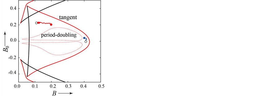
and , as shown in Figure 1. A stable fixed point exists in the shaded region surrounded by these bifurcations. Note that although the bifurcations curves are shown in Figure 1, we assume that the bifurcation structure is unknown. We only know the operating point at which the system has a stable fixed point. In the parameter region shown in Figure 1, our algorithm searches for the optimal parameter values, which means the farthest point from the three bifurcations. The simulation results are shown in Figure 1. Each colored circle is an initial parameter value of our six trials. From Figure 1, we can see that from any initial parameter value in the shaded region, our method finds the optimal parameter values denoted by the open circle corresponding to almost the center of the gray region. We consider that if the parameter value is set near this point, we can construct a system that is robust to parameter perturbation.
3.2. Continuous-Time System
An example of a continuous-time system is one described by Duffing’s equation:
 (19)
(19)
In this system, the Neimark-Sacker bifurcation never appears, because using Liouville’s theorem, the product of the two eigenvalues of the Jacobian matrix (Equation (12)) is given by . Typical phenomena observed in this system include nonlinear resonance and chaos due to successive period-doubling bifurcations [20] [21] .
Figure 2(a) shows the results of searching for parameter values with the maximum margin to bifurcations when . In this parameter region, there are at most three fixed points. Two of them are stable. The red bifurcation sets in Figure 2 are related to the fixed point which we treat here. Two initial values denoted by the red and blue circles in Figure 2(a) are chosen. From the blue point, our method can obtain a local optimal parameter value. From the red point, our method also reaches a local optimal parameter value: the farthest point from the bifurcations denoted by the red curves. To achieve a global search, we use the third parameter k. Figure 2(b) shows the results when changing the value of parameter k. The red circle indicates the initial parameter values when k = 0.05. From this point, we can find the optimal parameter values denoted by the open circle. In this case, our method can escape the complicated bifurcation area and reach parameter values far from them when k = 0.25.
4. Conclusion
We proposed a method of determining parameter values that are far from bifurcations in a parameter space. We

Figure 1. Bifurcation diagram and result of our method. A stable fixed point exists in the shaded region. The six colored points are the initial parameter values. From each initial value, we can obtain the optimal parameter values denoted by the open circle.
 (a)
(a)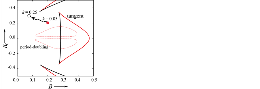 (b)
(b)
Figure 2. Results for Duffing’s equation. Red curves indicate the bifurcation sets of the fixed point corresponding to the non-resonant state. Chaotic states generated by successive period-doubling bifurcations exist in period-doubling bifurcation sets. (a) k = 0.05; (b) Using the third parameter k. Bifurcation sets are for k = 0.25.
described the method of calculating the normal vector to the bifurcation curves for periodic solutions. Our decision method uses the normal vector to find parameter values which are far from bifurcations. As illustrated examples, we showed the results of discrete-time and continuous-time systems. Our method could find optimal parameter values in both systems. Open problems are to extend the method so that it can deal with complicated bifurcation structures in a parameter plane and systems including uncertainty.
Acknowledgements
This research was supported by the Aihara Project, the FIRST program from JSPS, initiated by CSTP. This research was also supported by JSPS KAKENHI (23500367).
References
- Mackey, M. and Glass, L. (1997) Oscillation and Chaos in Physiological Control System. Science, 197, 287-289. http://dx.doi.org/10.1126/science.267326
- Glass, L. and Mackey, M. (1979) Pathological Conditions Resulting from Instabilities in Physiological Control System. Annals of the New York Academy of Sciences, 316, 214-235. http://dx.doi.org/10.1111/j.1749-6632.1979.tb29471.x
- Basso, M., Genesio, R. and Tesi, A. (1997) A Frequency Method for Predicting Limit Cycle Bifurcations. Nonlinear Dynamics, 13, 339-360. http://dx.doi.org/10.1023/A:1008298205786
- Berns, D.W., Moiola, J.L. and Chen, G. (1998) Predicting Period-Doubling Bifurcations and Multiple Oscillations in Nonlinear Time-Delayed Feedback Systems, Circuits and Systems I: Fundamental Theory and Applications. IEEE Transactions, 45, 759-763. http://dx.doi.org/10.1109/81.703844
- Chen, G., Moiola, J.L. and Wang, H.O. (2000) Bifurcation Control: Theories, Methods, and Applications. International Journal of Bifurcation and Chaos, 10, 511-548. http://dx.doi.org/10.1142/S0218127400000360
- Xie, Y., Chen, L., Kang, Y.M. and Aihara, K. (2008) Controlling the Onset of Hopf Bifurcation in the Hodgkin-Huxley Model. Physical Review E, 77, 061921. http://dx.doi.org/10.1103/PhysRevE.77.061921
- Overton, M.L. (1988) On Minimizing the Maximum Eigenvalue of a Symmetric Matrix. SIAM Journal on Matrix Analysis and Applications, 9, 256-268. http://dx.doi.org/10.1137/0609021
- Shapiro, A. and Fan, M.K.H. (1995) On Eigenvalue Optimization. SIAM Journal on Optimization, 5, 552-569. http://dx.doi.org/10.1137/0805028
- Imae, J., Furudate, T. and Sugawara, S. (1997) A Simple Numerical Method for Minimizing the Maximum Eigenvalues of Symmetric Matrices via Nonlinear Differential Equation Solvers. Transactions of the Japan Society of Mechanical Engineers, 63, 87-92.
- Dobson, I. (1993) Computing a Closest Bifurcation Instability in Multidimensional Parameter Space. Journal of Nonlinear Science, 3, 307-327. http://dx.doi.org/10.1007/BF02429868
- Kremer, G.G. (2001) Enhanced Robust Stability Analysis of Large Hydraulic Control Systems via a Bifurcation-Based Procedure. Journal of the Franklin Institute, 338, 781-809. http://dx.doi.org/10.1016/S0016-0032(01)00031-X
- Lu, J., Engl, H.W. and Schuster, P. (2006) Inverse Bifurcation Analysis: Application to Simple Gene Systems. Algorithms for Molecular Biology, 1, 1-16. http://dx.doi.org/10.1186/1748-7188-1-11
- Dobson, I. and Lu, L. (1993) New Methods for Computing a Closest Saddle Node Bifurcation and Worst Case Load Power Margin for Voltage Collapse. IEEE Transactions on Power Systems, 8, 905-913. http://dx.doi.org/10.1109/59.260912
- De Souza, A.C.Z., Canizares, C.A. and Quintana, V.H. (1997) New Techniques to Speed Up Voltage Collapse Computations Using Tangent Vectors. IEEE Transactions on Power Systems, 12, 1380-1387. http://dx.doi.org/10.1109/59.630485
- Monnigmann, M. and Marquardt, W. (2002) Normal Vectors on Manifolds of Critical Points for Parametric Robustness of Equilibrium Solutions of ODE Systems. Journal of Nonlinear Science, 12, 85-112. http://dx.doi.org/10.1007/s00332-001-0400-1
- Vahidi, B., Azadani, E.N., Divshali, P.H., Hessaminia, A.H. and Hosseinian, S.H. (2010) Novel Approach for Determination of Worst Loading Direction and Fast Prediction of Stability Margin in Power Systems. Simulation, 86, 729-741. http://dx.doi.org/10.1177/0037549709106507
- Tsumoto, K., Ueta, T., Yoshinaga, T. and Kawakami, H. (2012) Bifurcation Analyses of Nonlinear Dynamical Systems: From Theory to Numerical Computations, Nonlinear Theory and Its Applications. IEICE, 3, 458-476. http://dx.doi.org/10.1587/nolta.3.458
- Kawakami, H. and Kobayashi, K. (1979) Computer Experiments on Chaotic Solutions of x(t + 2) ax(t + 1) x2(t) = b. Bulletin of the Faculty of Engineering, Tokushima University, 16, 29-46.
- Mira, C., Fournier-Prunaret, D., Gardini, L., Kawakami, H. and Cathala, J.C. (1994) Basin Bifurcations of Two-Dimensional Noninvertible Maps: Fractalization of Basins. International Journal of Bifurcation and Chaos, 4, 343-381. http://dx.doi.org/10.1142/S0218127494000241
- Kawakami, H. (1984) Bifurcation of Periodic Responses in Forced Dynamic Nonlinear Circuits: Computation of Bifurcation Values of the System Parameters. IEEE Transactions on Circuits and Systems, CAS-31, 248-260. http://dx.doi.org/10.1109/TCS.1984.1085495
- Kitajima, H. and Kawakami, H. (1995) An Algorithm Tracing out the Tangent Bifurcation Curves and Its Application to Duffing’s Equation. IEICE Transactions on Fundamentals, J78, 806-810. http://dx.doi.org/10.1002/ecjc.4430790308