Open Journal of Fluid Dynamics
Vol.3 No.4(2013), Article ID:40402,9 pages DOI:10.4236/ojfd.2013.34031
Numerical Analysis of the Losses in Unsteady Flow through Turbine Stage
Institute of Power Engineering and Turbomachinery, Silesian University of Technology, Gliwice, Poland
Email: slawomir.dykas@polsl.pl
Copyright © 2013 Sławomir Dykas et al. This is an open access article distributed under the Creative Commons Attribution License, which permits unrestricted use, distribution, and reproduction in any medium, provided the original work is properly cited.
Received August 12, 2013; revised September 12, 2013; accepted September 20, 2013
Keywords: Turbine Stage; Stator; Rotor; Loss Coefficients
ABSTRACT
This paper presents an analysis of the operation of a stage of an aircraft engine gas turbine in terms of generation of flow losses. The energy loss coefficient, the entropy loss coefficient and an additional pressure loss coefficient were adopted to describe the losses quantitatively. Distributions of loss coefficients were presented along the height of the blade channel. All coefficients were determined based on the data from the unsteady flow field and analyzed for different mutual positioning of the stator and rotor blades. The flow calculations were performed using the Ansys CFX commercial software package. The analyses presented in this paper were carried out using the URANS (Unsteady Reynolds-Averaged Navier-Stokes) method and two different turbulence models: the common Shear Stress Transport (SST) model and the Adaptive-Scale Simulation (SAS) turbulence model, which belongs to the group of hybrid models.
1. Introduction
Aerodynamic losses in the flow through a turbine stage have an adverse impact on energy conversion efficiency. Obviously, due to the turbine stage specificity, the nature of these losses is unsteady. This is mainly related to the impact of the rotating rotor blade ring with the stationary stator blade ring and the intense turbulent phenomena which are responsible for blade losses [1]. These losses include as follows [2]:
• Profile losses which result from the friction of the viscous fluid against the blade surface, as well as from the finite thickness of the trailing edge, behind which the so-called aerodynamic wake is formed.
• Boundary losses which result from the effect that the near-wall layer and the medium flowing in the blade channel have on each other. The medium velocity in the near-wall boundary layer area, on the surfaces limiting the channel from top and bottom, is lower than in the remaining part of the channel. This leads to an imbalance of the forces resulting from the distribution of pressure and the deflection of the medium stream. Consequently, streamlines get deflected towards the base of the blade channel as well as in the direction of the convex (sucking) blade surface. The intensity of the described phenomena increases as the blade channel relative height becomes smaller.
• Losses resulting from incomplete feed. These losses occur in some steam turbines fed with high-parameter steam and in small gas turbines. They result from the fact that the stages used in such structures are not fed at full perimeter. Losses related to incomplete feed manifest themselves by gas being pushed out of the rotor channels which, due to the rotation of the rotor, found themselves before the fed nozzle segment and by the gas being mixed in areas at the edge of the feeding segment.
• Losses related to the cooling of the first stages of the gas turbine.
The energy dissipation phenomena occurring in a turbine stage are more and more often analyzed by means of the computational fluid dynamics (CFD) tools [3-5]. This paper presents the methodology and the results of CFD analyses comprising the unsteady flow in the turbine stage of an aircraft engine [6]. The use of the Ansys CFX commercial software package makes it possible to identify places where losses arise and in many cases allows their physical interpretation. The energy loss coefficient, the entropy loss coefficient and an additional pressure loss coefficient [1,2] were adopted to describe the losses quantitatively. The analyses presented in this paper were carried out using the URANS method and two different turbulence models: the common Shear Stress Transport
(SST) model and the Adaptive-Scale Simulation (SAS) turbulence model, which belongs to the group of hybrid models. The aim of the comparison of results obtained from analyses conducted with different turbulence models was to show whether the application of the SAS model, which is much more demanding in terms of equipment, is justified in the type of simulation under discussion.
2. Definitions of Loss Coefficients and Their Physical Interpretation
The expansion process in the turbine reaction stage (Figure 1) occurs both in the stator and rotor. It is an irreversible process accompanied by energy dissipation caused mainly by aerodynamic, thermodynamic and leakage-related losses.
Three types of loss coefficients [2] were used in this work to make a quantitative assessment of the losses arising in blade channels:
2.1. Entropy Loss Coefficient
The form of the entropy loss coefficient is derived directly from the definition of isentropic efficiency. This efficiency is defined for static parameters before and after the blade ring, where the difference between the values of real and isentropic enthalpy of the end of the expansion process is replaced with an increase in entropy, according to the second law of thermodynamics.
 (1)
(1)
 (2)
(2)
This coefficient is based on the theorem that the only reliable representation of losses occurring in the flow where an adiabatic process takes place is the increase in entropy [1]. This increase may have several sources. One of them is flow resistance resulting from movement of any viscous fluid. Apart from that, an increment in entropy may be caused by heat transfer at a finite temperature difference and by the unbalanced nature of some processes.
2.2. Energy Loss Coefficient
According to the energy conservation law (the first law of thermodynamics), the energy in a system remains constant; only its form may change. Therefore, the concept of energy loss is impossible from the physical point of view. However, it is common practice to use the energy loss coefficient in order to define the value of energy which does not participate in work generation. The

Figure 1. Expansion process in the turbine stage in the h-s chart.
form of this coefficient was derived from the energy conservation law, which states—for the stator blade ring —that total enthalpy is constant, while constant rothalpy is assumed for the rotor blade ring. For perfect gas it may eventually be written using total and static pressures.
 (3)
(3)
 (4)
(4)
2.3. Pressure Loss Coefficient
This is one of the most common loss coefficients in use. Its popularity results from the fact that determination of the parameters needed to find the coefficient is very easy. This feature is essential in experimental testing, where static and total pressure measurements are commonly applied and relatively easy to perform.
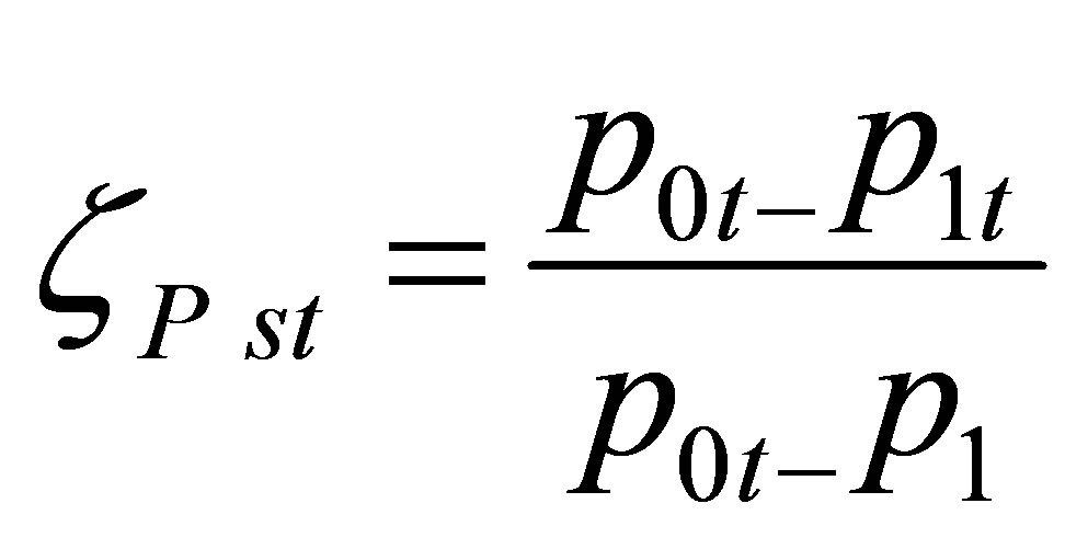 (5)
(5)
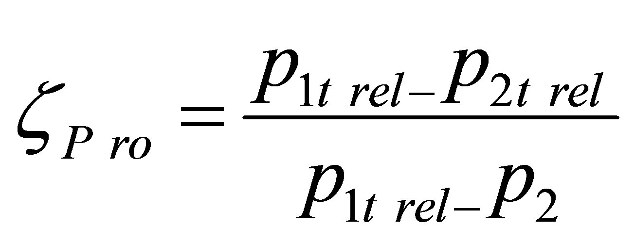 (6)
(6)
The pressure loss coefficient relates a loss of total pressure in the blade ring to the theoretical value of dynamic pressure that the medium would feature at the rotor outlet if loss pt did not occur. This loss may be caused by friction, presence of shock waves, etc.
3. Turbine Stage Geometry
This work presents an analysis of the unsteady flow in a gas turbine intended for the aircraft industry and described in [6]. The characteristic feature of the turbine is that it has just one stage, which distinguishes it from other turbines used in turbofan engines. Another important factor in the selection of the turbine stage was the publication of complete geometry of the blades and operating parameters of the analyzed stage in [6]. The stage under consideration is composed of 36 38.1 mm high stator blades located at an average radius of 469.9 mm and 64 rotor blades with the same height and radius of location. Due to the lack of data concerning the geometry of the tip seal of the rotor blades, a geometry was selected that is typical for this stage type. The geometry of the stage under analysis is presented in Figure 2.
An unstructured hybrid-type mesh composed of approximately 550 k nodes for each blade channel was used to discretize the computational domain. One channel for the stator blade ring and two channels for the rotor blade ring were assumed for the computations. This gives 1.7 M mesh nodes in total. The mesh of the tip seal of the rotor blades was generated as fully structured. It is composed of approximately 300 k nodes. While making the mesh, special care was taken to achieve accurate discretization in the near-wall boundary layers ensuring y+ ≈ 1.
The boundary conditions used in the analysis are presented in Table 1. The very high drop in pressure between the stage inlet and outlet makes the flow field much more complex. Two turbulence models—the Shear Stress Transport (SST) and the Scale-Adaptive Simulation (SAS) [7] were used in the performed numerical simulations.
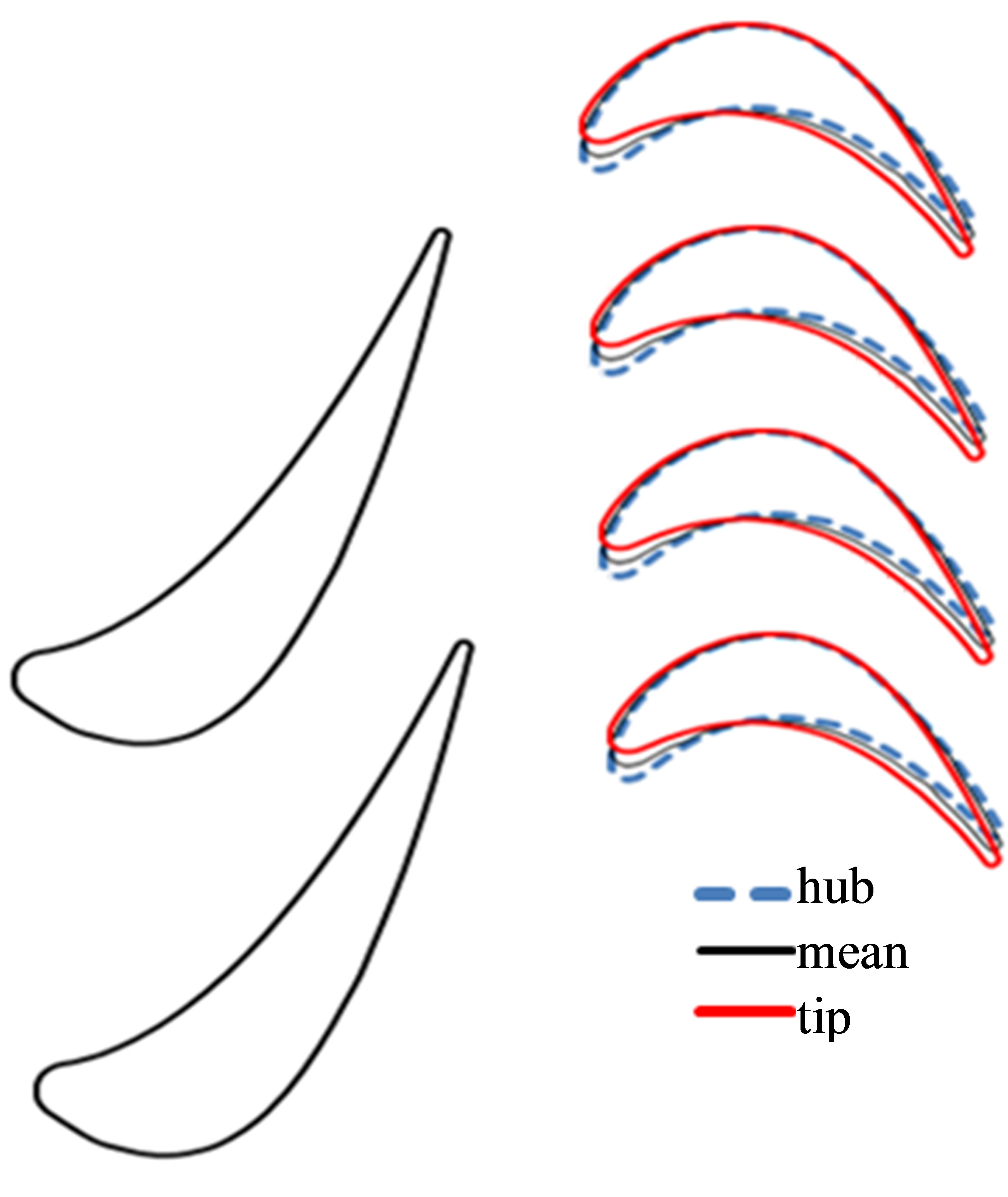

Figure 2. Geometry of the analyzed turbine stage.

Table 1. Data assumed for the reference analysis.
The stage-type interface between the stator and rotor was used for steady computations. Its characteristic feature is “averaging” parameters in the circumferential direction. It is also better than an alternative frozen rotor-type interface. For the unsteady analysis, the transient rotor-stator-type interface was applied.
4. Calculation Results
The performed analyses of the unsteady flow field make it possible to determine aerodynamic losses and the impact of the mutual positioning of the stator and rotor on their magnitude. The application of the Ansys CFX package for numerical analyses made it possible to obtain curves of loss coefficients depending on the relative height of the flow channel. In this case, the individual parameters of the medium taken for the analysis were averaged in terms of mass in the circumferential direction. While finding loss coefficients, the parameters with subscript 2 denoting the medium after the rotor were determined in the channel extension. This is to make it possible to take account of the losses resulting from the presence of the blade wake and shock waves. The mutual positioning of the stator and rotor blades for individual steps is presented in Figure 3.
4.1. Entropy Loss Coefficient Analysis
Figure 4 presents distributions of the entropy loss coefficient along the channel height. In the case of the stator blade (Figures 4(a) and (c)) the value of zS,st for almost 80% of the blade height is less than 0.05 (5 percentage points). This proves that the energy conversion level in the stage under analysis is high. The entropy loss coefficient reaches the highest values on the surfaces limiting the channel from top and bottom. This is caused by the occurrence of boundary losses in these areas. The values of these losses at the channel top are smaller than at the bottom, which results from the bigger width of the blade channel. Moreover, higher values of the Mach number occur in the bottom part of the channel than in the remaining parts. The blade channel under analysis features a confusor section and therefore, to reach the velocity of Ma > 1, the medium has to be subjected to Prandtl Meyer expansion. Theoretically, this is an isentropic process. However, the change in the flow direction related to it leads to the creation of shock waves which are the source of losses.
Comparing Figure 4(a) with Figure 4(c), which present the distribution of the entropy loss coefficient for the stator channel, it can also be seen that the coefficient values are higher for calculations performed using the SST turbulence model. The differences reach 0.005, which, for example in a new unit designing process, is a significant value.
The minimum and maximum values of the entropy loss coefficient are achieved for both turbulence models used for the same time step. However, the values of coefficient zS,st obtained for the two models differ from each other substantially. For intermediate time steps the discrepancies are even greater.
The distribution of the entropy loss coefficient for the rotor channel is more complex (Figures 4(b) and (d)). The high value of zS,ro in the upper part of the channel is the effect of, among others, the seal operation. The medium leaving the seal cavity generates secondary flows [2] which lead to a considerable increase in the entropy loss coefficient in the area of 0.8 - 1 of the channel height (Figure 5). In the case of the stator, the decrease in the entropy loss coefficient in this region was much more abrupt and small values of the coefficient were obtained already at 0.95 of the channel height. The data presented in Figures 4(b) and (d) also
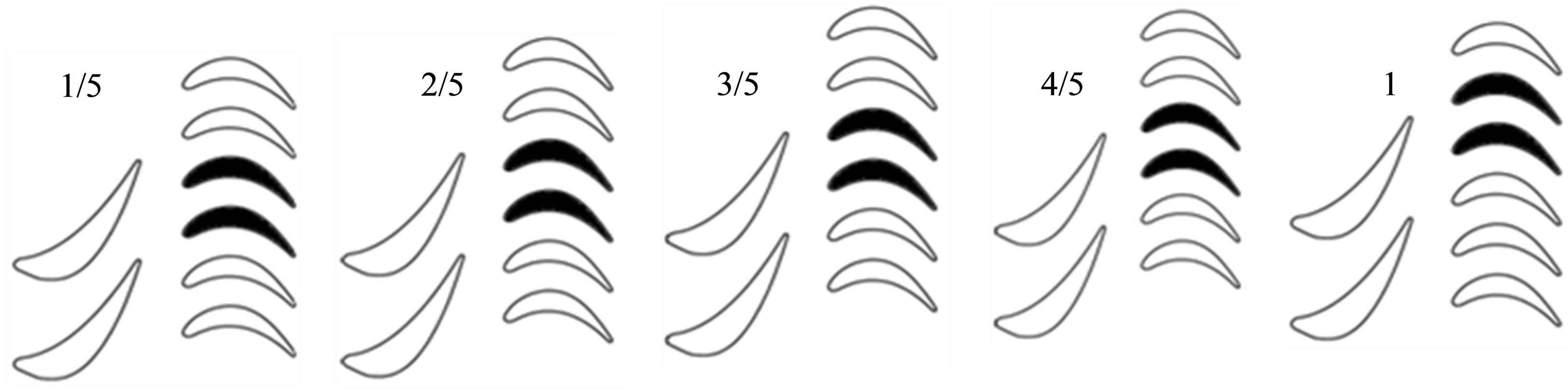
Figure 3. Mutual positioning of the stator/rotor blades for individual time steps.
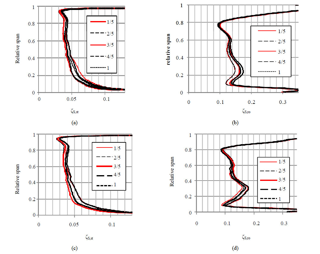
Figure 4. Distribution of the entropy loss coefficient for reference analyses (low temperatures): (a) stator, SST; (b) rotor, SST; (c) stator, SAS; (d) rotor, SAS.
indicate that the entropy loss coefficient for almost the entire height of the channel assumes values higher than 0.1. This proves that the efficiency of the analyzed rotor blade ring is much lower than that of the stator.
At 0.3 of the relative height of the channel coefficient zS,ro reaches values bigger than 0.15. This is related to the substantial increment in the entropy of the medium in the trailing edge area. At this height the increment is clearly bigger than in the remaining part of the channel (Figure 6). Also in the area of ~0.3 of the relative height of the channel the biggest changes in the loss coefficient occur depending on the mutual stator/rotor positioning. These changes probably result from the unsteady nature of the blade wake vortices and from the shock waves arising in the trailing edge region.
In the case of the rotor blade ring channel, a big discrepancy is observed between the entropy loss coefficient values calculated for the results obtained using different turbulence models. The difference is especially noticeable in the area of 0.2 - 0.3 of the relative height of the
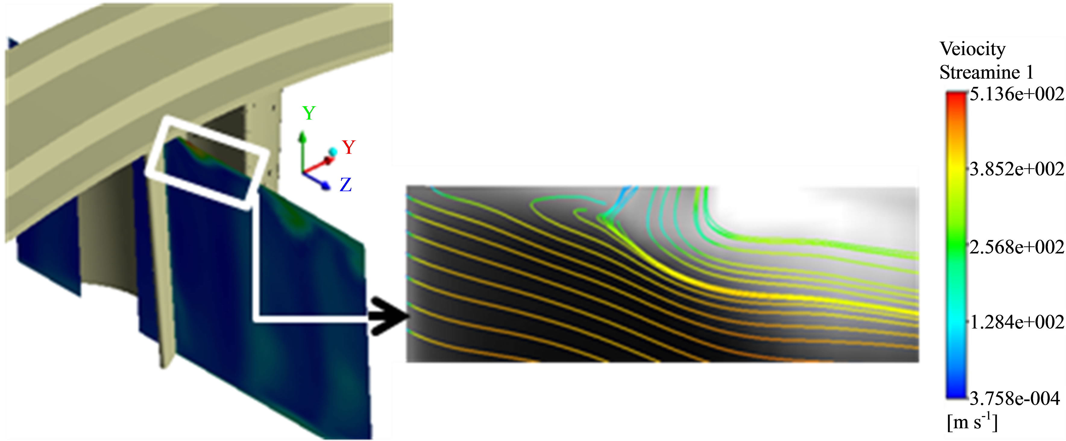
Figure 5. Generation of reverse flows in the area where the medium leaving the seal mixes with the main flow.
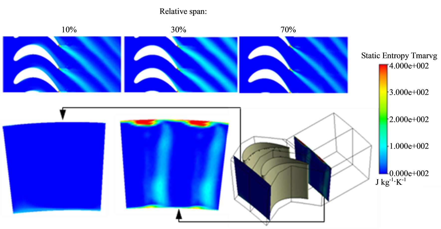
Figure 6. Distribution of static entropy in the rotor channel; reference analysis; SAS turbulence model.
channel, where the values assumed by coefficient zS,ro are high. The SAS model located the mentioned area at a bigger height of the channel compared to the SST model. Moreover, for the SST turbulence model, the values of zS,ro in this area diverge less from the values assumed in other regions of the blade. The fluctuations in the values of zS,ro are in this region higher for the SST model and reach 0.03.
4.2. Energy Loss Coefficient Analysis
Figures 7(a) and (c) present distributions of the energy loss coefficient along the height of the stator blade. The amplitude of fluctuations in the values of zEn,st decreases rather uniformly with the blade height. Above 0.97 of the channel relative height the curves formed for individual time steps coincide. The biggest changes in the energy loss coefficient occur at 0.2 of the channel relative height, where they reach 0.035.
In the case of the SST turbulence model, an intersection of zEn,st curves occurs for subsequent time steps 2/5 and 3/5. This proves that there is a phase shift in changes in the energy loss coefficient for areas above and below the point of intersection. As this point is situated in the upper part of the blade, where amplitudes of fluctuations in the values of zEn,st are slight, the phase shift mentioned above will have little effect on “smoothing” the amplitudes of changes in the loss coefficient calculated for the entire stator blade ring. It is the big amplitude of the changes in the bottom part of the channel that has a decisive impact on how the coefficient evolves.
Figures 7(b) and (d) show distributions of values of the energy loss coefficient calculated for the channel
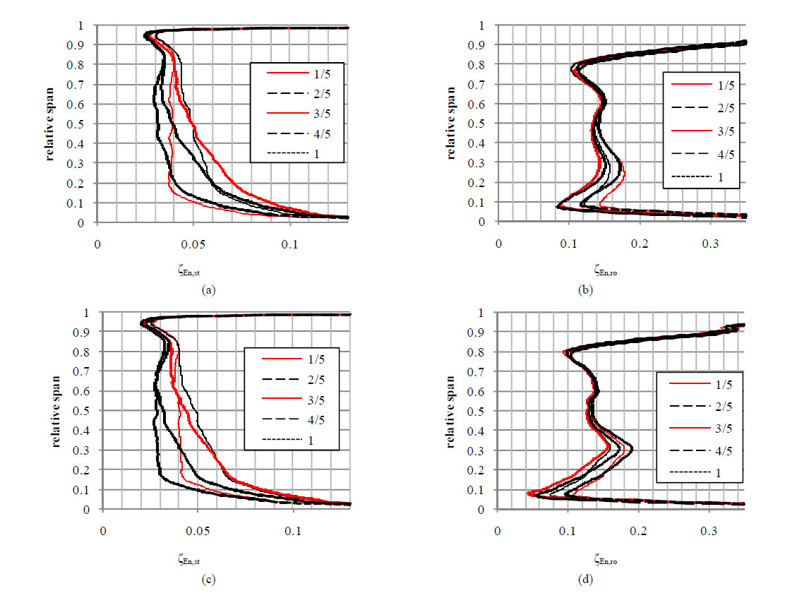
Figure 7. Distributions of the energy loss coefficient for reference analyses (low temperatures): (a) stator, SST; (b) rotor, SST; (c) stator, SAS; (d) rotor, SAS.
of the rotor blade ring. The biggest difference between the values of zEn,ro for both turbulence models is visible in the bottom part of the channel. At ~0.1 of the blade relative height it exceeds 0.03. In this area there is also a difference between the values of fluctuations in zEn,ro. These fluctuations feature slightly bigger amplitudes in the case of results obtained using the SST turbulence model.
At 0.3 of the channel relative height (where previously an especially big increment in the entropy of the medium was observed in the trailing edge region) the SAS turbulence model gave a much larger increase in the energy loss coefficient than that modelled by the SST model. This may indicate a significant impact of the turbulence phenomena in this region, which are better mapped by the SAS model, on the energy loss coefficient value.
In the figures presenting distributions of the energy loss coefficient values for the rotor channel no intersections of curves are observed for time steps subsequent to each other.
In this situation the fluctuations in average values of zEn,ro calculated for the entire blade can be seen quite clearly.
Moreover, it can be noticed that low values of zEn,st correspond to high values of zEn,ro. The changes in values of the energy loss coefficient for individual blade rings will in a way balance each other, reducing fluctuations in the average value of the loss coefficient calculated for the entire stage.
4.3. Pressure Loss Coefficient Analysis
Figures 8(a) and (c) present distributions of the pressure loss coefficient for the channel of the stator blade ring. Their shape is similar to the shape of zEn,st curves because both coefficients are functions of the same parameters of the medium. As it was the case for the energy and entropy loss coefficients, the values of zP,st are smaller for the calculation results obtained using the SAS turbulence model. The differences between the results of the two models reach 0.02 (time step “1” and 0.2 of the channel relative height).
The range of changes in the values of the pressure loss coefficient for the stator channel decreases with its height. At 0.2 of the channel relative height fluctuations in the values of zP,st amount to as much as 0.055. At the same time it can be seen that the changes in values of the pressure loss coefficient along the channel entire length do not run in the same direction. This is proved by several intersections of curves for time steps 1/5, 2/5 and 3/5.
Figures 8(b) and (d) present distributions of the pressure loss coefficient for the rotor blade ring. The most significant difference between the values of this coefficient for the SST and SAS turbulence models occurs in the bottom part of the flow channel. Here, for the SAS model, the pressure loss coefficient assumes values smaller even by 0.07. At the same time, fluctuations in the values of zP,ro for this particular turbulence model (SAS) feature bigger amplitudes. The maximum range of the fluctuations is achieved at 0.1 of the channel relative height, where it assumes the value of 0.11. Fluctuations in zP,ro in the upper part of the blade are very slight. In principle, a noticeable amplitude occurs only at the point of deflection of the curves, at 0.8 of the channel relative height. A change in the value of zP,ro in this region may result from unsteady operation of the seal.
Considering the impact of the mutual stator/rotor positioning on the zP,ro value, a drop in value of the pressure loss coefficient can be observed for the first three time steps (mutual stator/rotor positions). In the next steps the value rises. This change takes place smoothly along the channel entire height, which is proved by the fact that there is no clear intersection of curves formed for two time steps subsequent to each other.
5. Conclusions
Based on the results of the numerical analyses performed for the gas turbine stage, it can be stated that the SST turbulence model obtained higher values of loss coefficients compared to the SAS model. This statement is correct for the part of the channel where there are no intense phenomena resulting in energy dissipation. In the upper part of the rotor channel, where the impact of the seal is significant, and at 0.3 of the channel relative
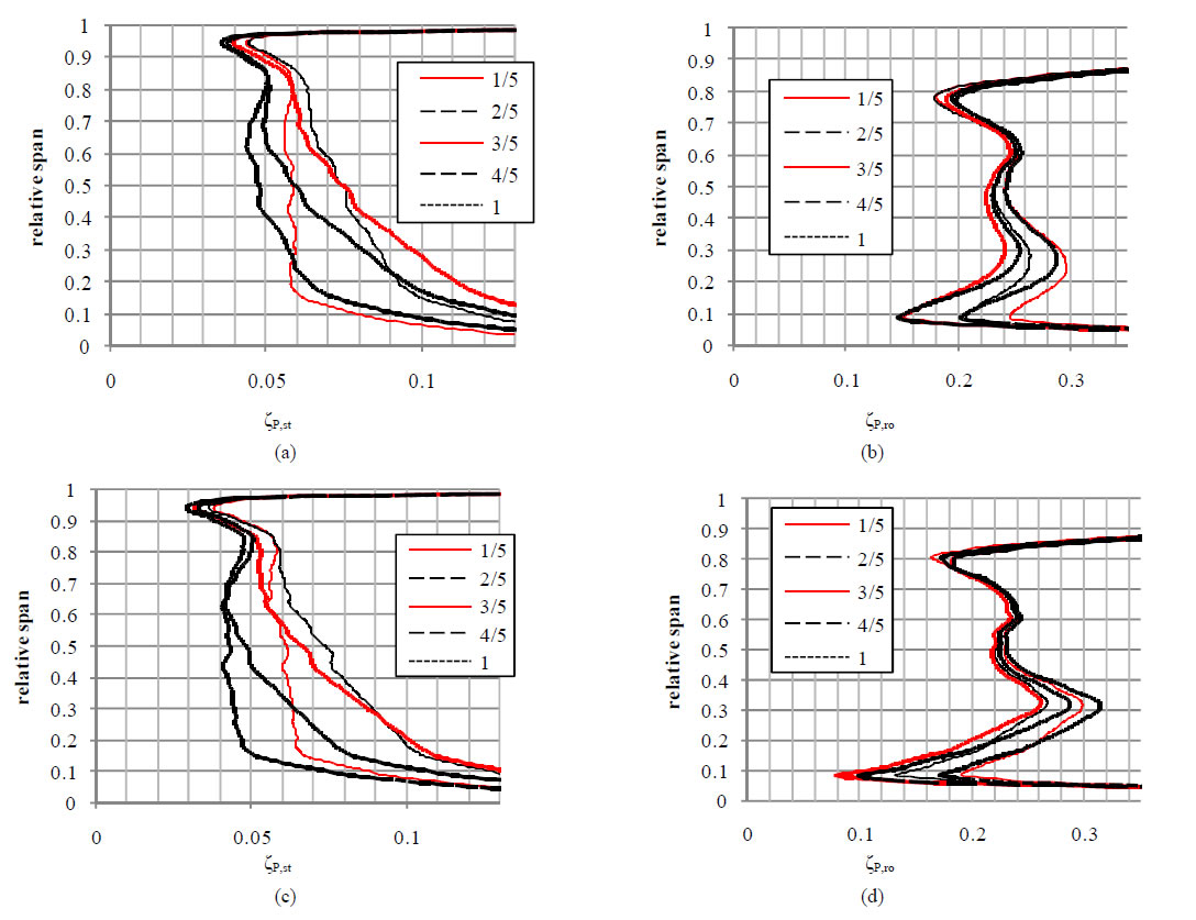
Figure 8. Distributions of the pressure loss coefficient for reference analyses (low temperatures): (a) stator, SST; (b) rotor, SST; (c) stator, SAS; (d) rotor, SAS.
height, where an especially big increment in entropy occurs, the values of the loss coefficients obtained for the SAS turbulence model are higher. This probably results from the fact that the turbulent processes taking place in these areas are mapped better by the hybrid Scale-Adaptive Simulation (SAS) turbulence model.
Comparing the two turbulence models, attention should also be drawn to the shape of the deflection of the curves in the area at ~0.3 of the blade relative height. Here, the curves representing changes in loss coefficients vary mildly for the SST model, whereas for the SAS turbulence model a considerable refraction of the curves occurs. Thus the area of high values of the loss coefficient for the SAS model comprises a much smaller part of the channel.
Intersections of curves for time steps subsequent to each other were observed for the energy loss coefficient and the pressure loss coefficient calculated for the stator channel. This proves that there is a phase shift in the direction of the changes in the coefficient value on both sides of the intersection of the curves, which leads to a reduced fluctuation in the average value of the loss coefficient calculated for the entire channel.
For all loss coefficients under analysis, the low values in the rotor region correspond to their high values in the region of the stator blade channel. This levels out the fluctuations in the values of individual coefficients within the entire stage.
6. Acknowledgements
The authors would like to thank the Polish Ministry of Science and Higher Education for the financial support for the research project UMO-2011/01/B/ST8/03488.
REFERENCES
- J. D. Denton, “Loss Mechanisms in Turbomachines,” Journal of Turbomachinery, Vol. 115, No. 4, 1993, pp. 621-656. http://dx.doi.org/10.1115/1.2929299
- N. Wei, “Significance of Loss Models in Aerothermodynamic Simulation for Axial Turbines,” Doctoral Thesis, Royal Institute of Technology.
- S. Dykas, W. Wróblewski and H. Łukowicz, “Prediction of Losses in the Flow through the Last Stage of LowPressure Steam Turbine,” International Journal for Numerical Methods in Fluids, Vol. 53, No. 6, 2007, pp. 933-945. http://dx.doi.org/10.1002/fld.1313
- P. Lampart, “Investigation of Endwall Flows and Losses in Axial Turbines, Part I. Formation of Endwall Flows and Losses,” Journal of Theoretical and Applied Mechanics, Vol. 47, No. 2, 2009, pp. 321-342.
- W. Wróblewski, A. Gardzilewicz, A. Dykas and P. Kolovratnik, “Numerical and Experimental Investigation of Steam Condensation in LP Part of Large Power Turbine,” Journal of Fluids Engineering, Trans, ASME, Vol. 131, No. 4, 2009, pp. 1-11.
- T. P. Moffit, E. M. Szanca and W. J. Whitney, “Design and Cold-Air Test of Single-Stage Uncooled Core Turbine With High Work Output,” NASA Report TP-1680, 1980.
- F. R. Menter, “Two-Equation Eddy-Viscosity Turbulence Models for Engineering Applications,” AIAA Journal, Vol. 32, No. 8, 1994, pp. 1598-1605. http://dx.doi.org/10.2514/3.12149
Symbols
z: loss coefficient h: specific enthalpy, J·kg−1
p: pressure, Pa s: specific entropy, J/kg−1·K−1
ϰ: adiabatic exponent
Subscripts
0: stator inlet 1: stator/rotor interface 2: rotor outlet En: energy rel: rotating reference frame ro: rotor s: entropy st: stator t: total