Open Journal of Fluid Dynamics
Vol.3 No.3(2013), Article ID:37039,8 pages DOI:10.4236/ojfd.2013.33021
A Comparison of the Ghost Cell Technique for Front Tracking Method
1College of Aerospace Engineering, Nanjing University of Aeronautics and Astronautics, Nanjing, China
2College of Science, Nanjing University of Aeronautics and Astronautics, Nanjing, China
3College of Science, PLA University of Science and Technology, Nanjing, China
Email: wangdonghong@nuaa.edu.cn
Copyright © 2013 Donghong Wang et al. This is an open access article distributed under the Creative Commons Attribution License, which permits unrestricted use, distribution, and reproduction in any medium, provided the original work is properly cited.
Received June 4, 2013; revised July 3, 2013; accepted July 17, 2013
Keywords: Compressible Multifluid; Front Tracking Method; Riemann Problem
ABSTRACT
The treatment of moving material interfaces and their vicinity is very important for compressible multifluids. In this paper, we propose one type of ghost fluid method based on Riemann solutions for front tracking method. The accuracy of the interface boundary condition is discussed for the gas-gas Riemann problem. It is shown that the solution of the ghost fluid method approximates the exact solution to second-order accuracy in the sense of comparing to the exact solution of a Riemann problem at the material interface. Numerical examples suggest that the present scheme is able to handle multifluids problems with large density differences and has the property of reduced conservation error.
1. Introduction
The dynamics of interfaces separating different fluids in compressible flows is of interest in several scientific fields as diverse as astrophysics and geophysics. It is also of significant importance in many engineering applications. A relatively dominant difficulty for simulating compressible multi-medium flow is the treatment of moving material interfaces and their vicinity. In general, there are two basic issues that need to be taken into account. One is to capture the interface location and topological changes accurately. Researchers can take all kinds of effective measures such as volume of fluid method [1] or level set technique [2] or front tracking technique [3] to deal with it. The other is to faithfully simulate the interface state including physical nonlinear wave interaction occurring at the interface.
The ghost fluid method (GFM) based techniques [4-8] provide us simple and flexible ways for handling multimedium flows with immiscible material interfaces. A closely related ghost cell level set method [4] was proposed by Fedkiw. But the GFM is problem-related and not suitable for some cases like high speed jet impacting [5]. To take into consideration the influence of both, wave interaction and material properties on the interfacial evolution led to the development of a modified ghost fluid method (MGFM) [5,7]. Wang [8] also presented a real ghost fluid method (RGFM) by predicting the flow states for the real fluid nodes just next to the interface and the ghost fluid nodes using the Riemann problem solver.
For the GFM [4-8], the level set technique [2] is employed to capture the moving interface. However, they can be used with other techniques for tracking the interface. Recently, Hao [9] and Terashima [3] extend Tryggvason’s method [10] using Fedkiw’s ghost fluid method [4] to handle compressible flows. Based on Riemann solutions, front tracking method combined with MGFM and RGFM had been discussed [11].
In this paper, a relatively class of GFM based on Riemann solutions is developed. One solves a system of a two-shock approximation to the Riemann problem for prediction of the condition at the interface. Then one uses the predicted pressure and velocity as those for the ghost fluid and the real fluid nodes just next to the interface. The isobaric entropy is employed at the interface to fix the real fluid density at node just next to the interface to suppress the possible “overheating” and also to assign density for the ghost fluid. The RGFM is one of this type of GFM. We combine the GFM with a front tracking method (GFM-FT). The front tracking method [12] is used here. The accuracy of the interface boundary condition is discussed for the gas-gas Riemann problem.
The conservation errors of this class of GFM and MGFM are analyzed for FT method. Numerical tests show that the GFM-FT has the property of reduced conservation error comparing to MGFM-FT.
2. Equations
The Euler equations governing one-dimensional compressible flows are written as
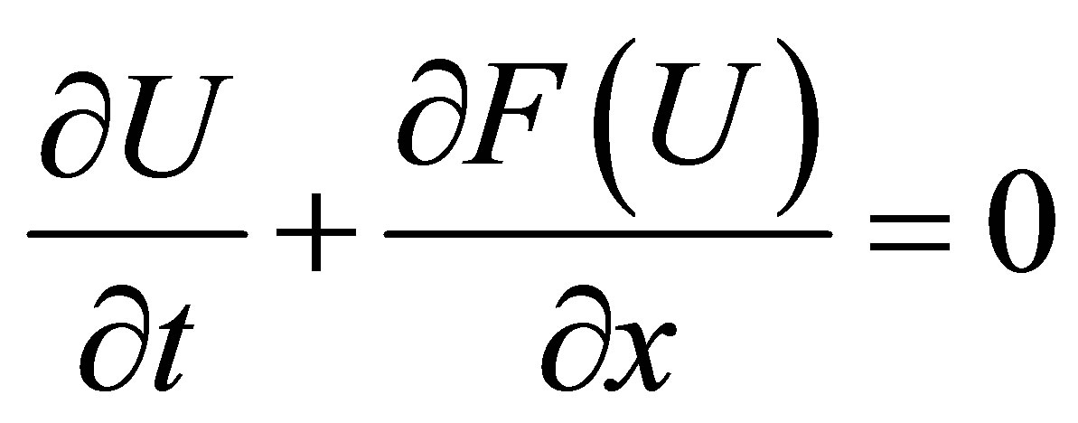 (1)
(1)
where
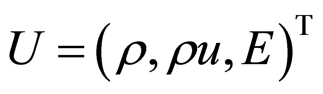 ,
, 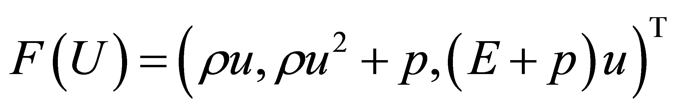 Here
Here  is the density,
 ![]() is the velocity,
is the velocity, ![]() is the pressure, and
is the pressure, and  is the total energy per unit volume. The total energy is the sum of internal energy and kinetic energy,
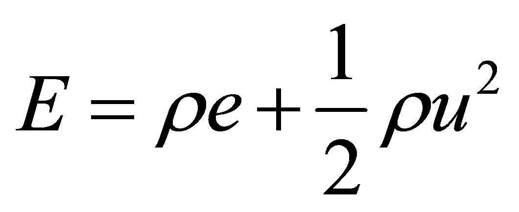 , (2)
, (2)
where ![]() is the internal energy per unit mass.
is the internal energy per unit mass.
For closure of Equation (1), the equation of state (EOS) is required. The EOS for compressible gases and water can be expressed in the following consistent form as
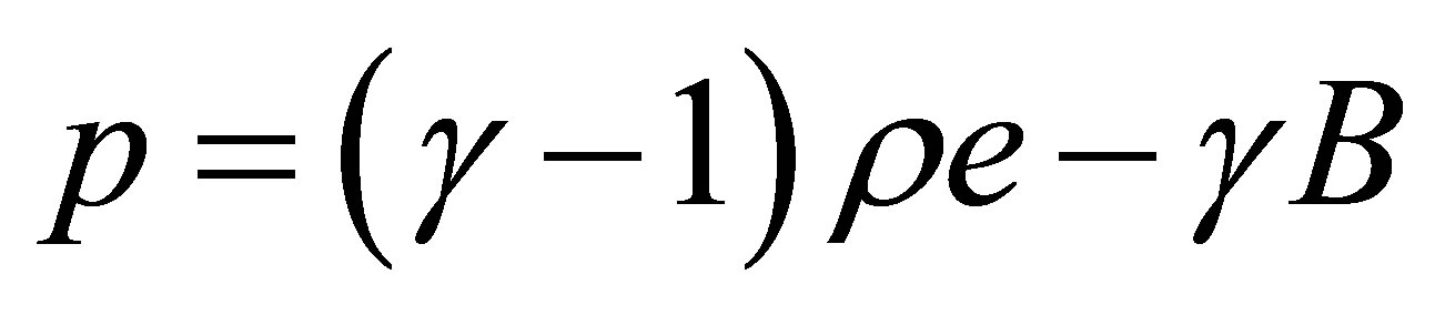 , (3)
, (3)
where  and
and  are treated as constants. For the air,
  ,
, . For the water medium (Tait’s equation),
  ,
, .
.
3. Tracking Fluid Interfaces
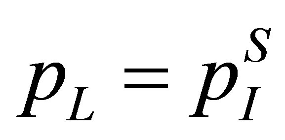
Suppose that the interface lies between node i and node i + 1. To define the Riemann problem at the interface, the two initial constant states of the Riemann problem are simply given as  and
and . Once the Riemann problem is defined, the two shock Riemann problem solver [5] can then be employed to provide intermediate interfacial states—
 (pressure),
  (velocity), and
  and
and  (the densities on the left and right sides of the interface). Now, having determined the interface velocity
  and its spatial location, the interface is moved between
 ![]() and
and .
.
4. Ghost Fluid
The initial conditions for the governing Equation (1) are given as
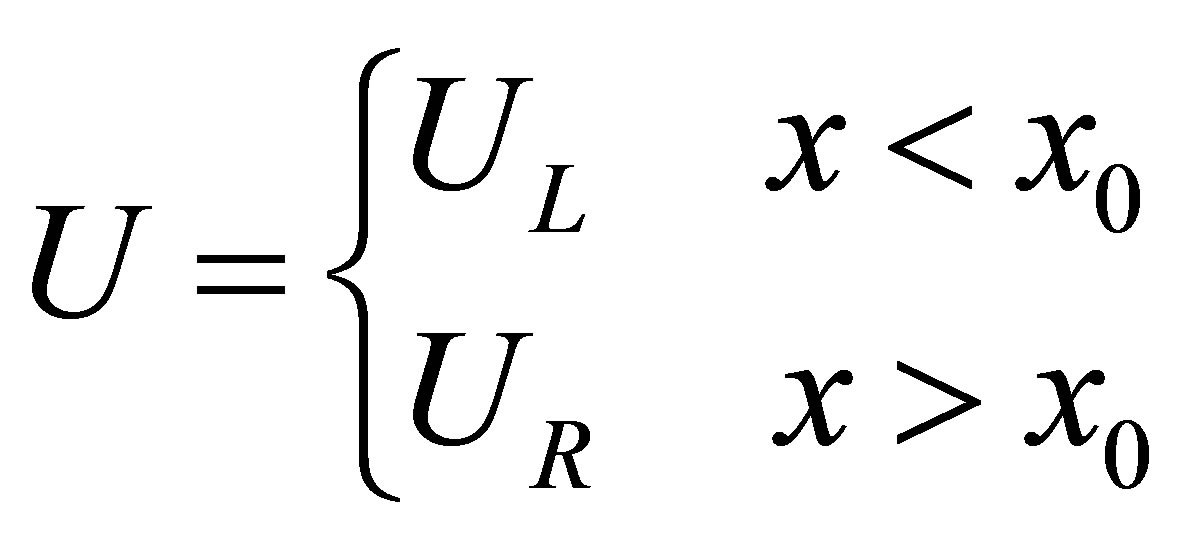 . (4)
. (4)
Regardless of the numerical scheme used, an algorithm based on the GFM essentially consists of solving two separate Riemann problems in the two respective single media with one-sided ghost fluid. One is in medium 1 (on the left side of the interface) with the initial conditions of
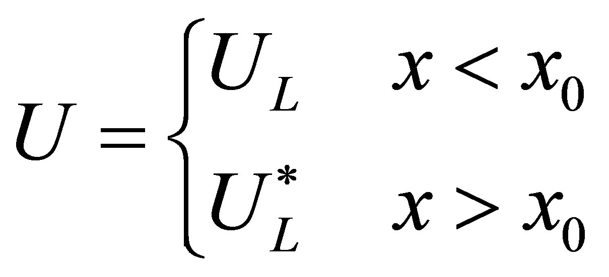 (5)
(5)
and it solves from the grid point 1 on the left-end to the ghost point, The other is in medium 2 (on the right side of the interface) with the initial conditions of
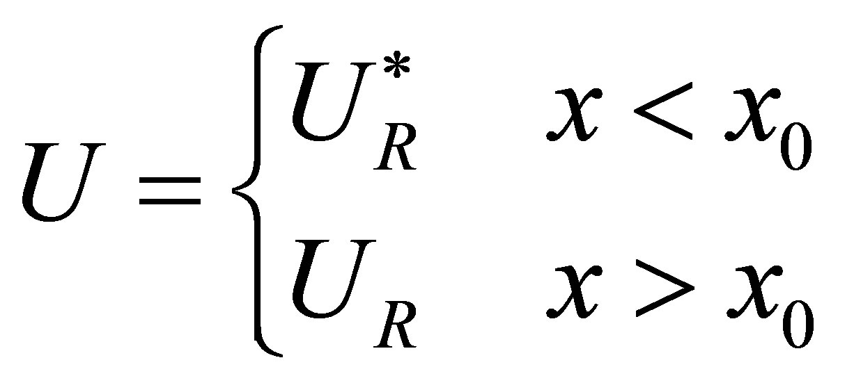 (6)
(6)
and it solves from the ghost point to the end point on the right. Here, “*” indicates the fluid states have been replaced by the ghost fluid states.
With the method of characteristics, we have the relations
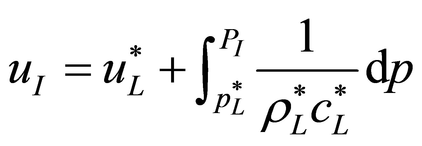 (7)
(7)
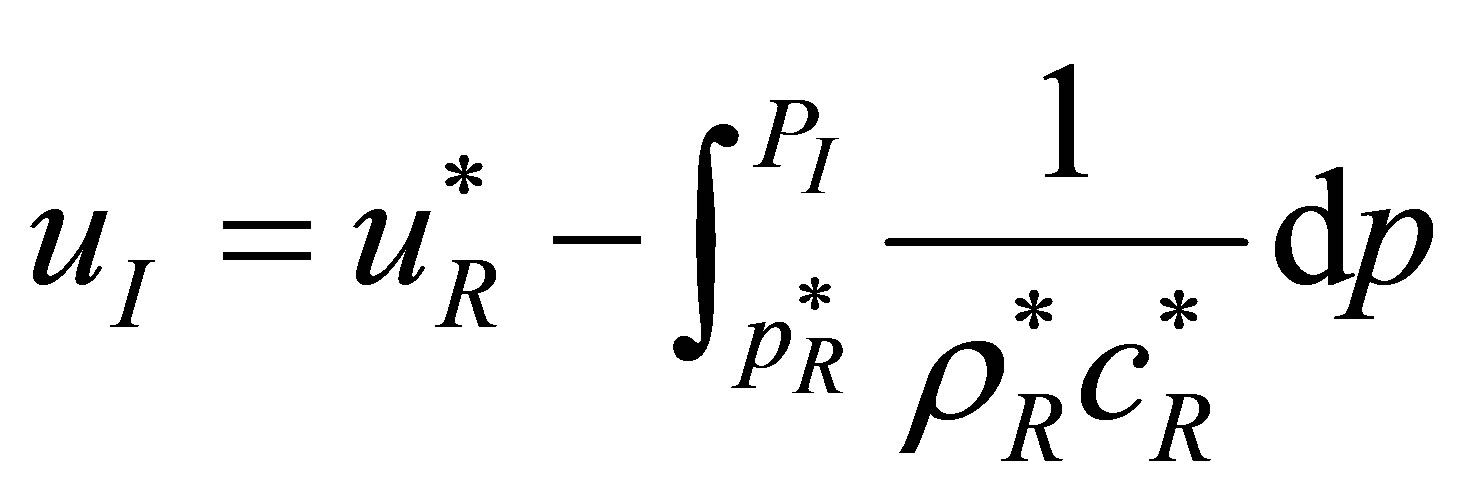 (8)
(8)
where  and
and  are the densities and sound speeds of the ghost fluid.
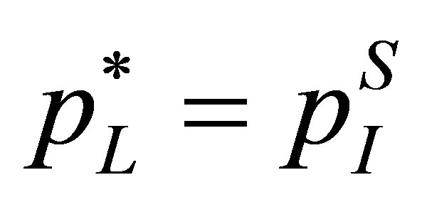
The ghost fluid states can be chosen by solving Equation (7) and (8). The simplest case is that the ghost fluid pressure be defined as the interface pressure, i.e.
 . (9)
. (9)
Hence the integral in Equation (7) and (8) become zero and the ghost fluid velocity is
 . (10)
Furthermore, one can find that any ghost fluid density can satisfy Equation (5) or (6).
For Equation (5) or (6), Hu [6] had considered two algorithms. The focus is on defining the ghost fluid states while the pressure and velocity in the real fluid side are taken for granted, except for the correction made to the density at the real fluid nodes next to the interface to overcome the overheating. Indeed, the real fluid states next to the interface instead of the ghost fluid states should be predicted by solving a Riemann problem [8]. This will result in the complete redefinition of the real fluid next to the interface. In doing so, one will find that the nonphysical reflection for the shock impedance matching problem can be greatly and further suppressed.
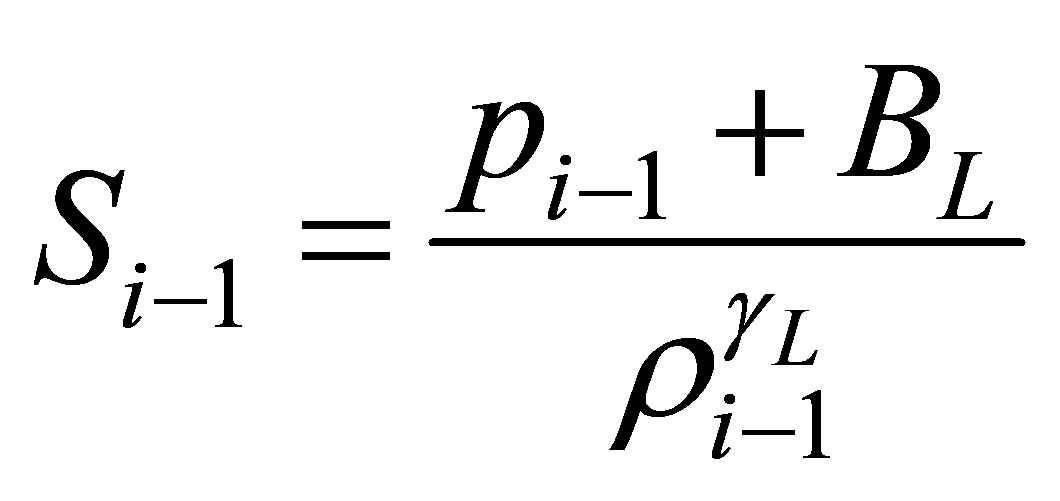
For medium 1, we take  and
and  as the pressure and velocity at nodes
 ,
,  ,
,  , For medium 2, we also take
  and
and  as the pressure and velocity at nodes
 ,
, . The ghost fluid density is based on isentropic fixing. Here, we shall consider two cases:
Case 1: For medium 1, the predicted isobaric entropy
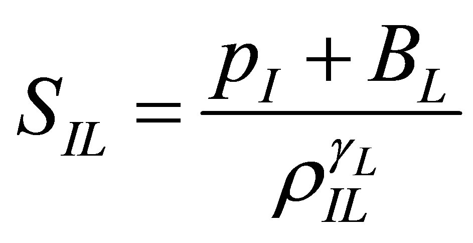 at the interface is employed to fix the real fluid density at point i and the ghost fluid density at point
 ,
, . A similar procedure is used for computation in medium 2. This is the RGFM [8] which can be seen from Figure 1.
Case 2: For medium 1, one employs isobaric entropy
 to fix the real and ghost fluid density.
The rest of the procedures are the same as those for Case 1. We take this method as SGFM which can be seen from Figure 2.
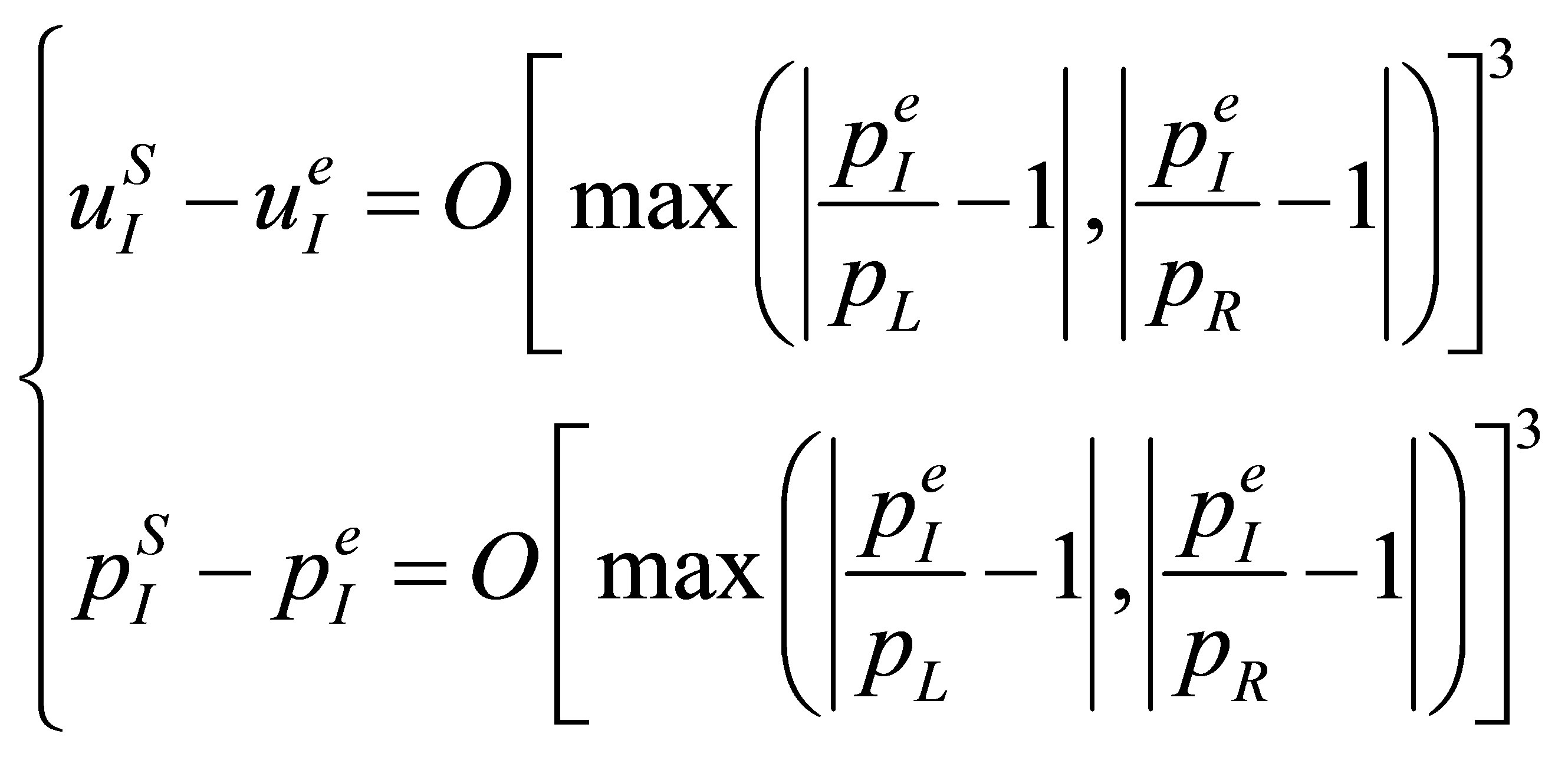
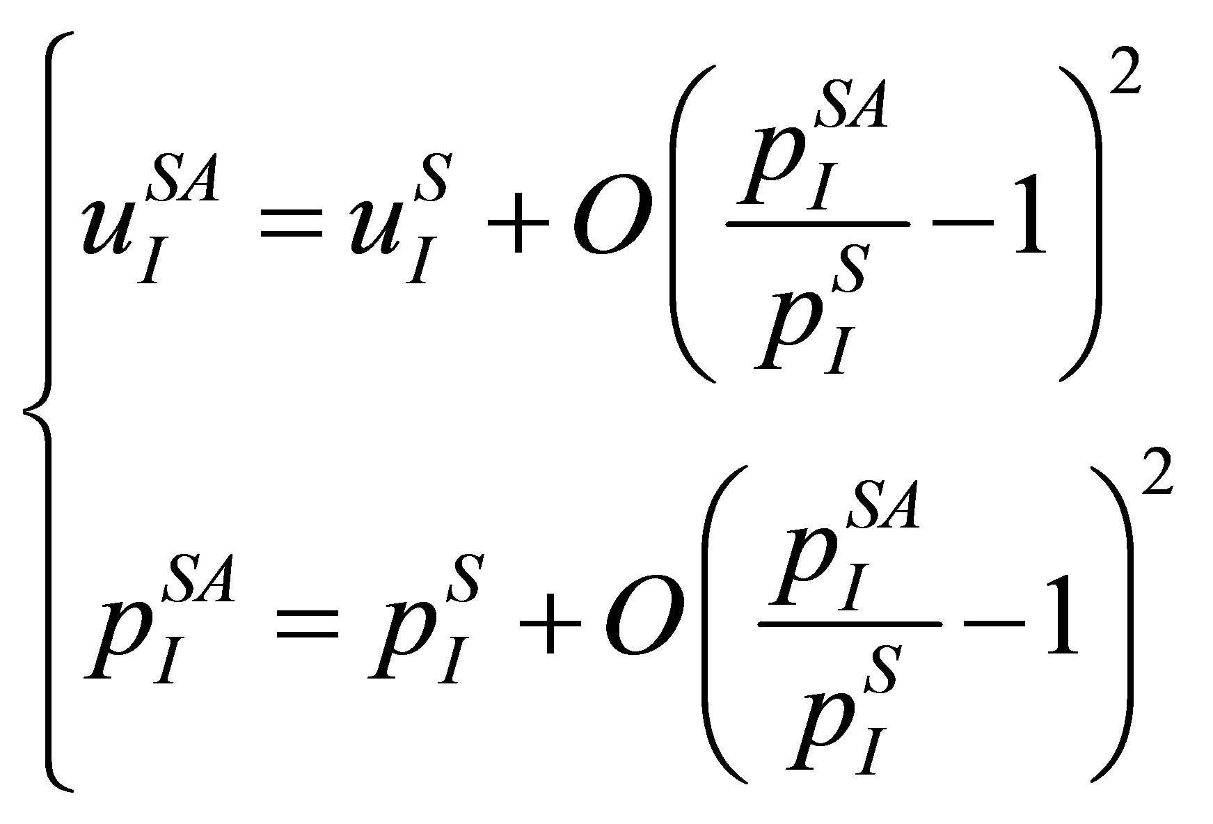
5. The Accuracy of SGFM and RGFM
We only consider the gas–gas Riemann problem. The accuracy of MGFM had been discussed [13]. It may be noted that the accuracy discussed should be interpreted as how accurate the boundary conditions are implicitly imposed at the material interface and how accurate the interface states are approximated by the GFM technique; it should not be explained or analyzed as the accuracy of final numerical solution and/or the numerical scheme used because the detailed numerical scheme is never involved in the discussion. An approximate Riemann problem solver (ARPS) based on a doubled shock structure is used for the Riemann problem. For the SGFM
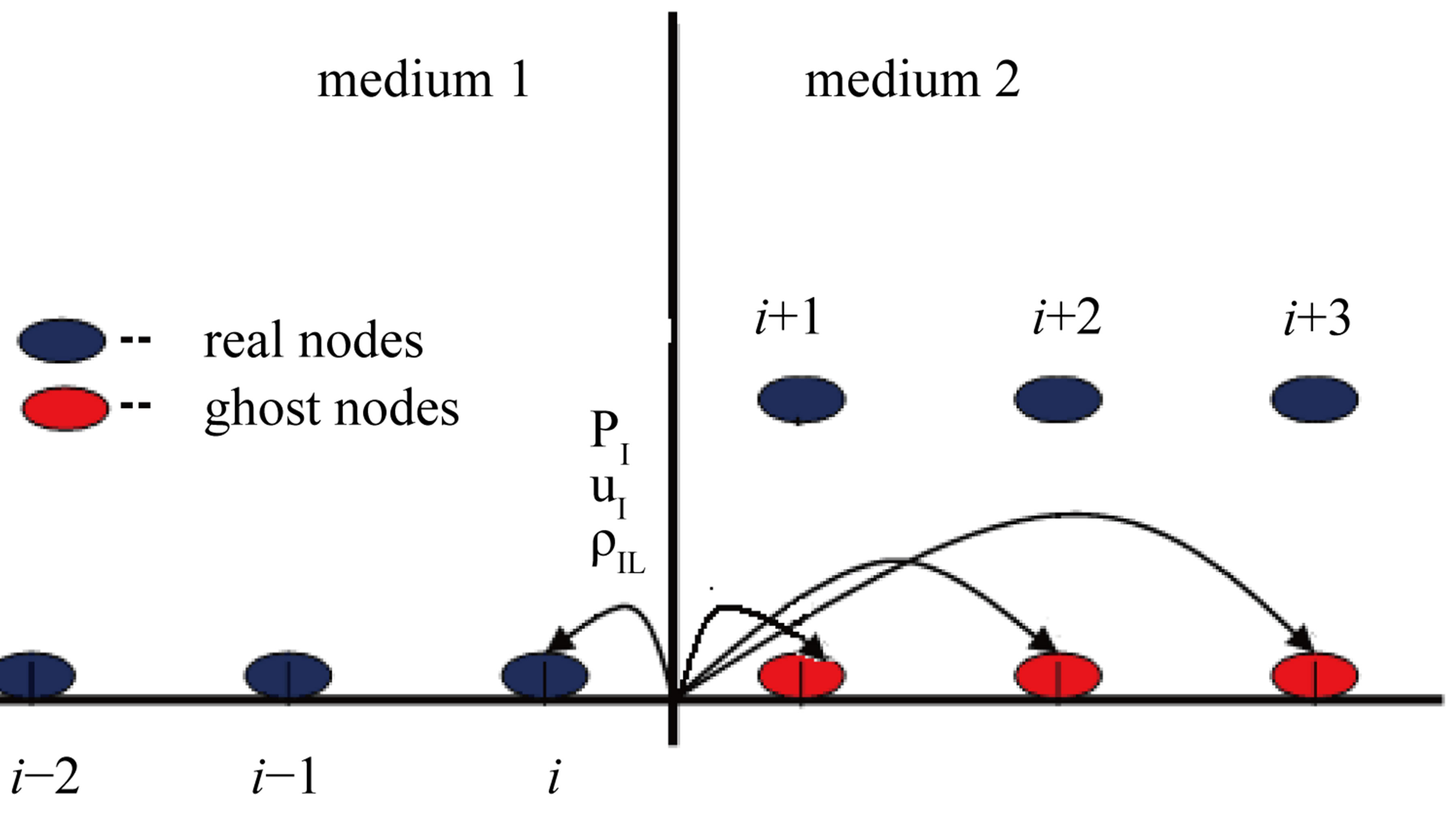
Figure 1. Isobaric fixing for RGFM.
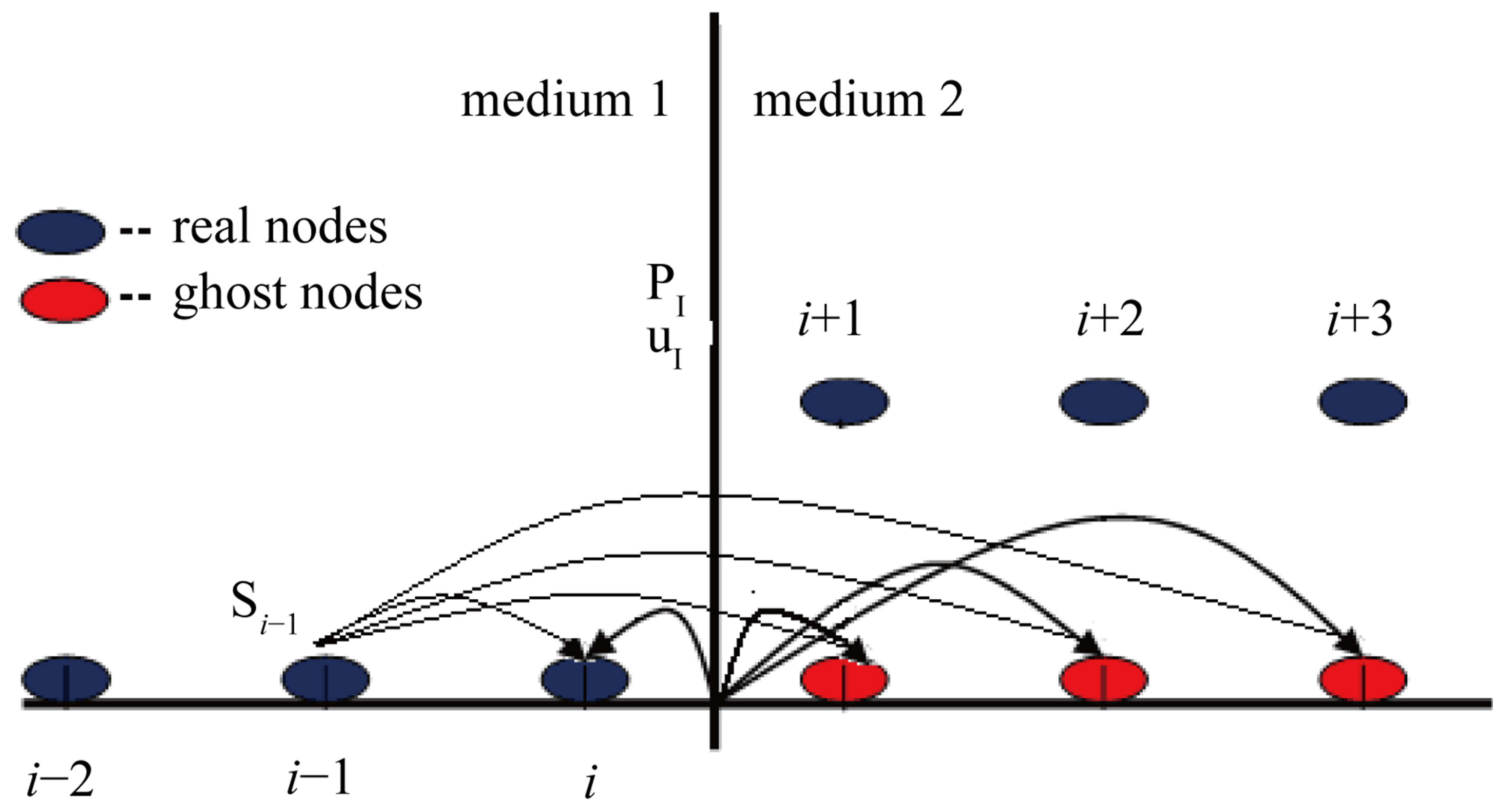
Figure 2. Isobaric fixing for SGFM.
applied to the Riemann problem (4), the following error estimations are held [13]
 (11)
(11)
Here,  and
and  are the exact interfacial pressure and velocity,
  and
and  are the interfacial pressure and velocity from ARPS.
For SGFM, we have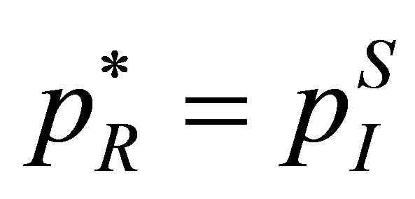 ,
,  ,
,  and
and , the pressure and velocity at the real fluid node next to the interface are also redefined. Following conclusions are held for the SGFM when applied to the Riemann problem (4).
Theorem 1. The following error estimates are held for the respective GFM Riemann problems (5) and (6) using the SGFM
(A) 
(B) 
(C) 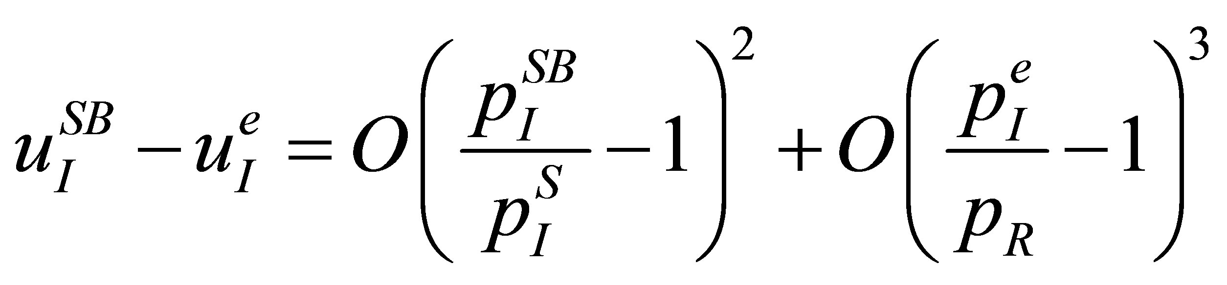
(D) 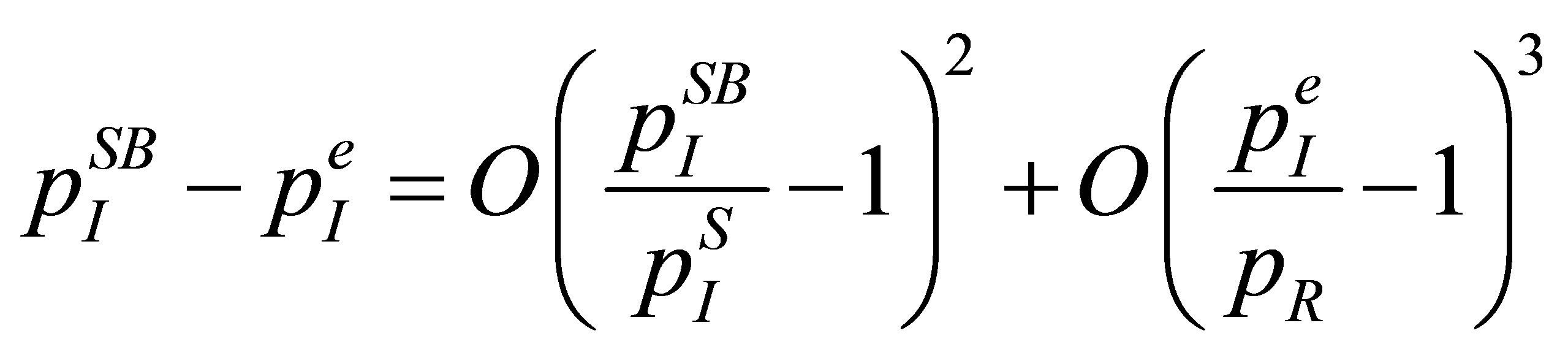
 and
and 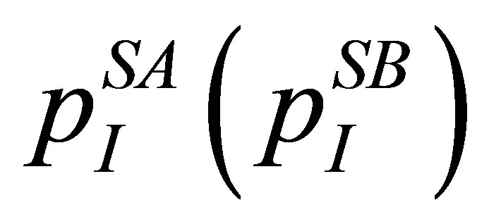 are the exact interfacial velocity and pressure of the GFM Riemann problem (5) and (6) using the SGFM.
Proof: Applying Theorem 2.1 [13] to the GFM Riemann problem (5), one gets
 (12)
(12)
According to SGFM, one has ,
, 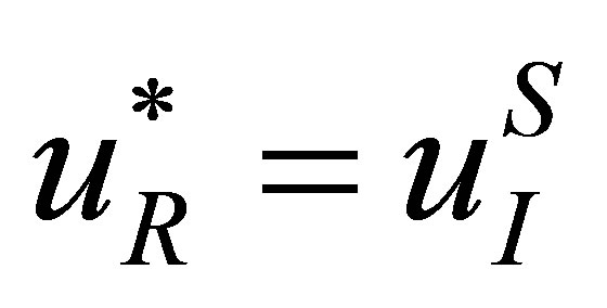 and the pressure and velocity at the real fluid node next to the interface are
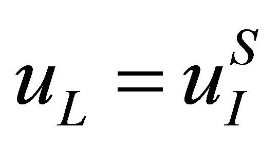 ,
, . Equation (12) can be expressed as
 (13)
(13)
Using Equation (11), one has
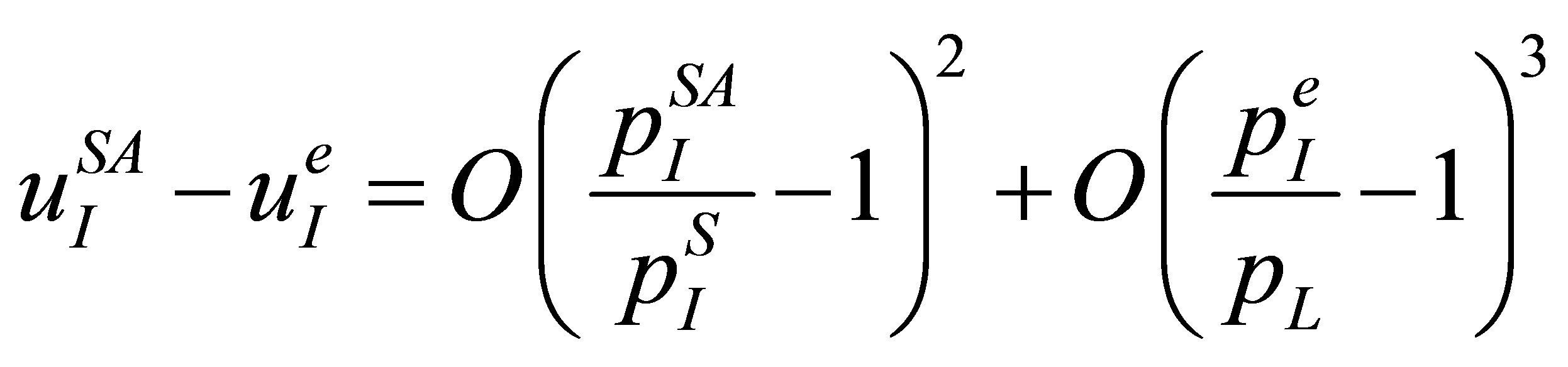 (14)
(14)
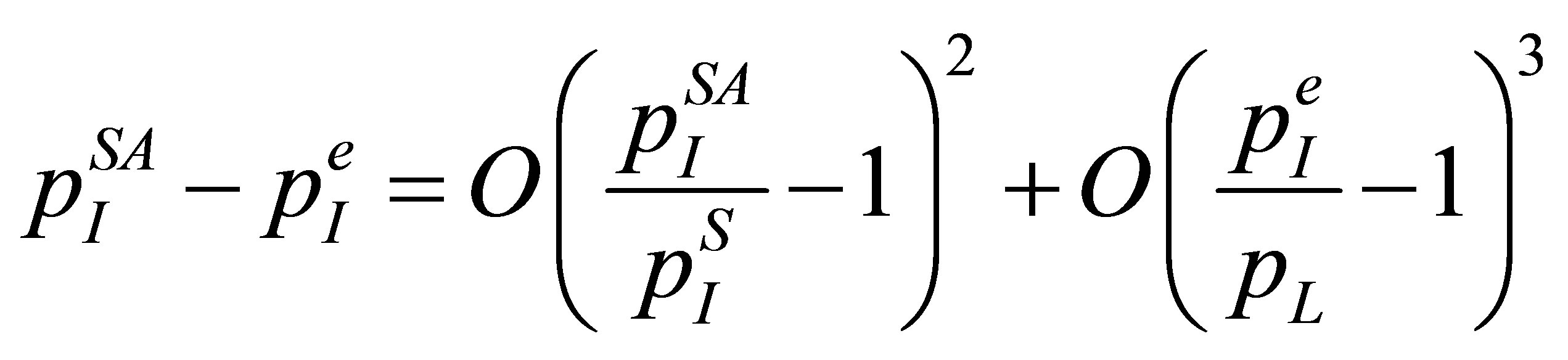 (15)
(15)
For the GFM Riemann problem (6), in a similar way, one can show that error estimates (C) and (D) in Theorem 1 are true.
The states of the ghost cell for RGFM are in accord with those for SGFM except the density. So Theorem 1 is also true for RGFM. It is shown that the solution of the SGFM and RGFM approximate the exact solution to at least second-order accuracy in the sense of comparing to the exact solution of a Riemann problem at the material interface.
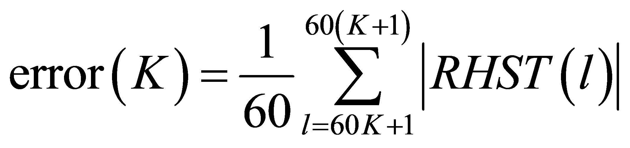
6. The Conservation Errors
Both overall conservation and conservation for each medium will be evaluated using Equation (1) over the computational domain . We denote RHSL(n), RHSR(n) and RHST(n) as the conservation errors for the medium on the left, right side of the interface and over the whole computational domain, respectively, as follows:
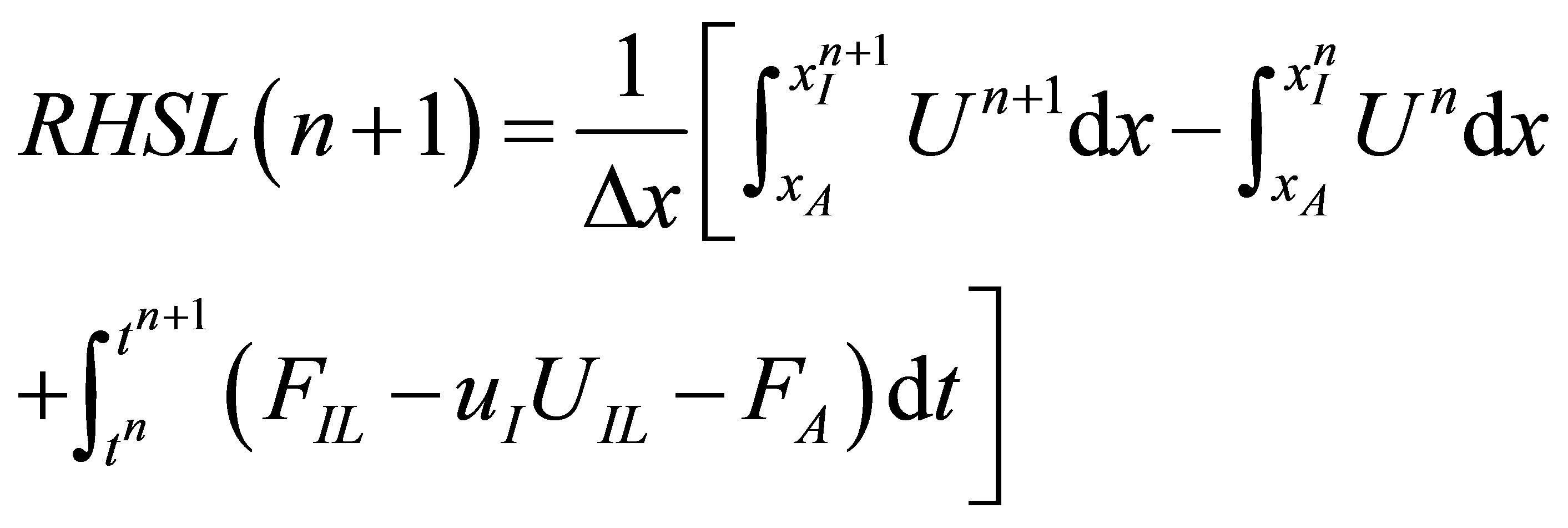 (16)
(16)
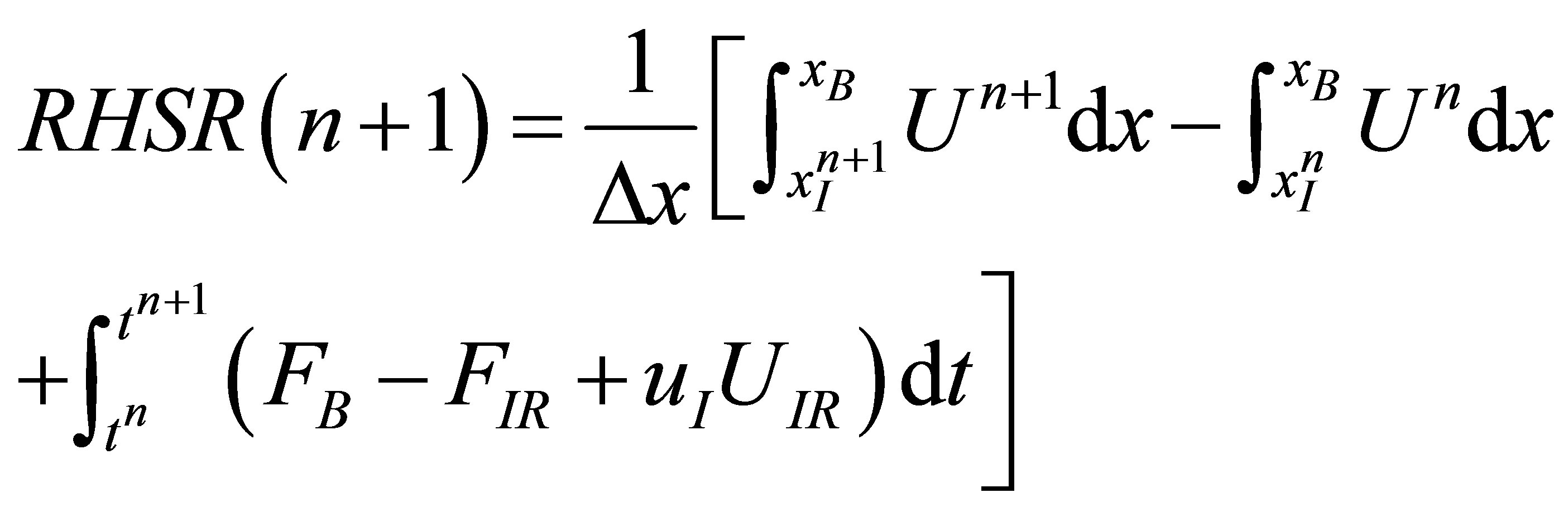 (17)
(17)
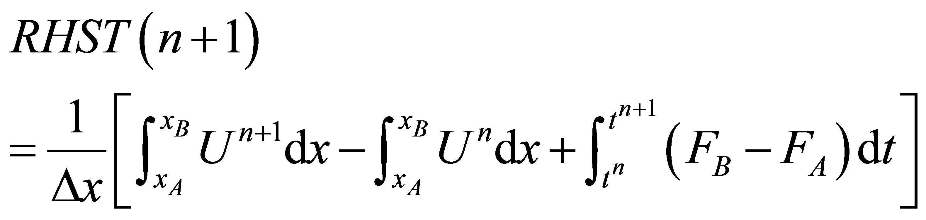 (18)
(18)
Here,  denotes the interface position;
  and
and  are fluxes at
  and
and , respectively.
  and
and  are fluxes at the respective left and right sides of the interface.
The overall average conservation error can be taken as
 (19)
(19)
We shall use two cases to study the conservation errors of the RGFM and SGFM.
Case 1: a strong shock impacting on an air-air interface (i.e., Problem 1 in Section 7)
From Table 1, it is clear that very large errors incur for the MUSCL-based MGFM-FT in the first 60 steps for this specific case, while these are suppressed very well by the MUSCL-based SGFM-FT and RGFM-FT. The conservative errors of the RGFM-FT and SGFM-FT are tend to zero faster than the MGFM-FT.
Case 2: This is a problem of a water column separated by the air and oscillating in the middle of a closed tube [8]. The problem is sketched in Figure 3. The initial status of the air and water are defined as
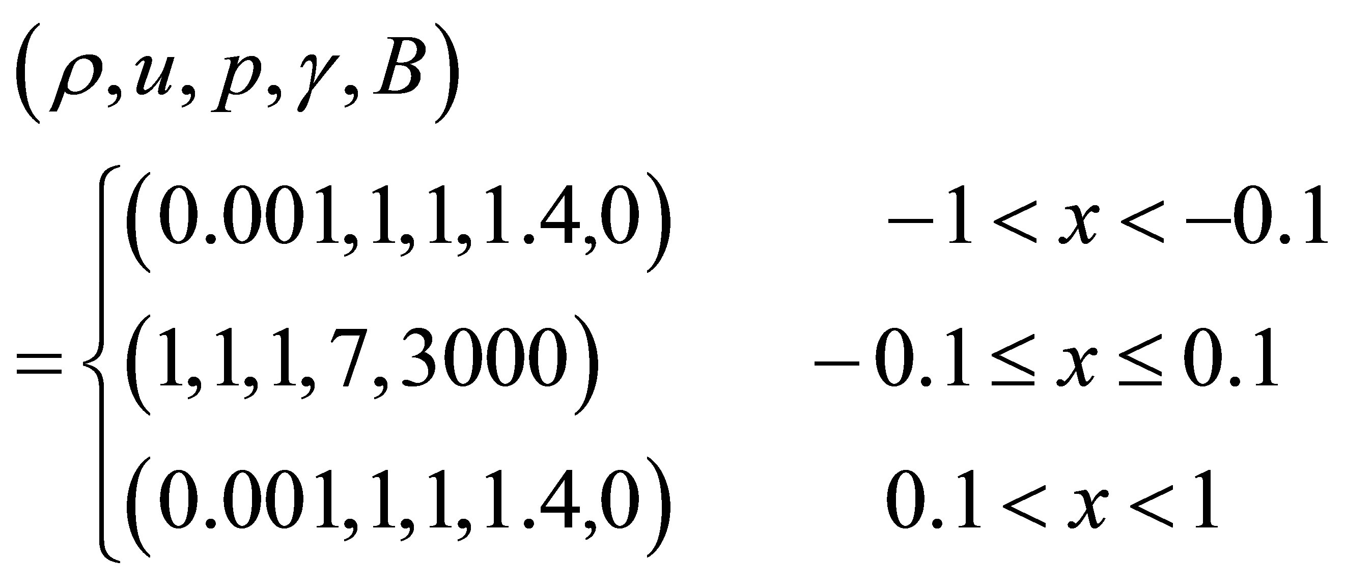
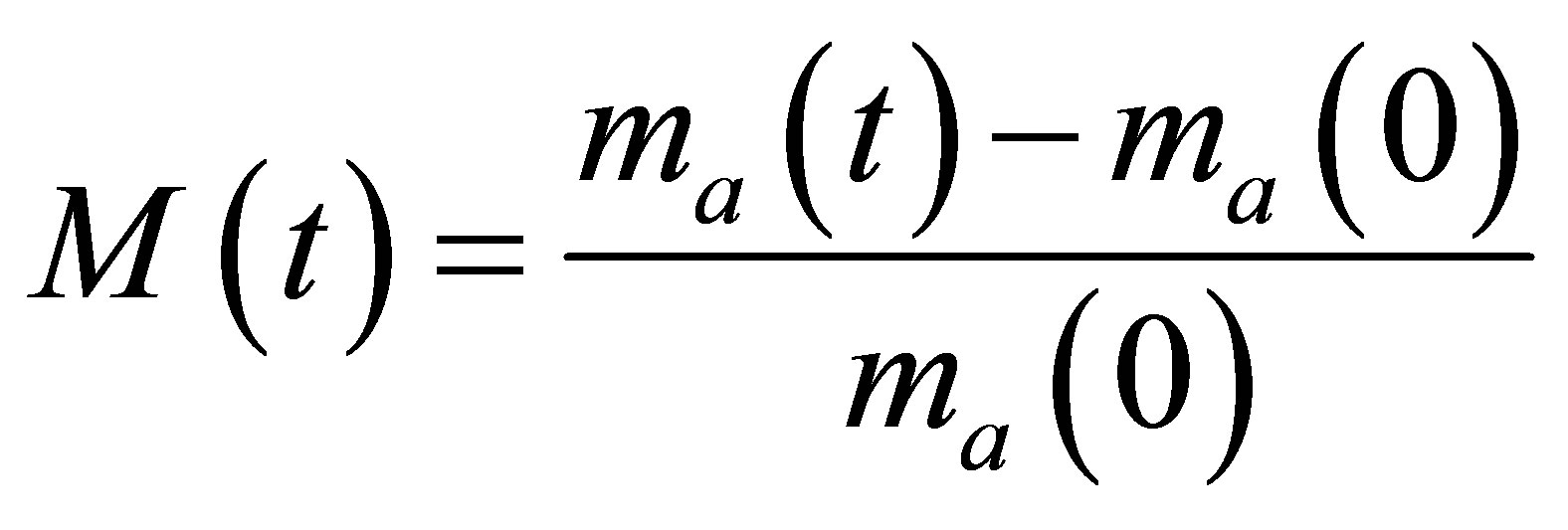
With the fluids moving to the right, the air on the left of the water column expands while the air on the right of the water column is compressed. The pressure decreases at the former and increases at the latter; this leads to the deceleration and eventually stagnation of the fluids in the tube. Then the fluids move in the reverse direction due to the pressure gradient, and so on with the water column oscillating. Pressure waves are evident in the tube due to the impact of the air on the end boundaries and interacttion with the water column. The conservation errors of the air mass M(t) are given as
 (20)
(20)
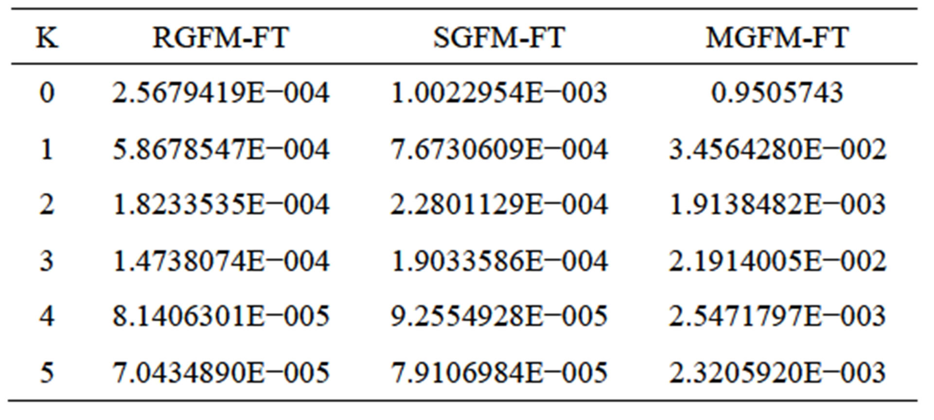
Table 1. The conservation errors of the RGFM-FT, SGFMFT and MGFM-FT.
Figure 3. Initial status of the oscillating water column problem.
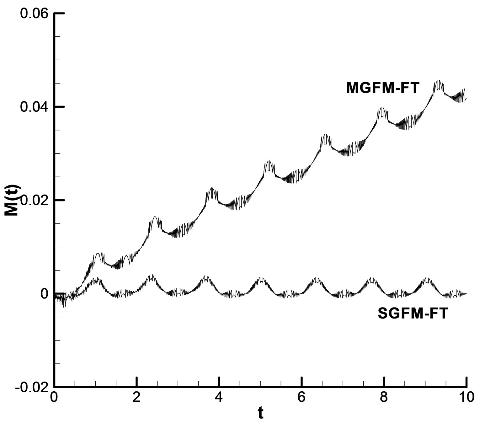
where  is the total mass of the air in the tube at time t. It can indeed be observed that the conservation errors associated with the air mass appear to be oscillating similar to that observed in [8]. Figure 4(a) depicts that MGFM has an oscillatory M(t) with a much larger trend of net conversion of the air mass into water when
 (a)
(a)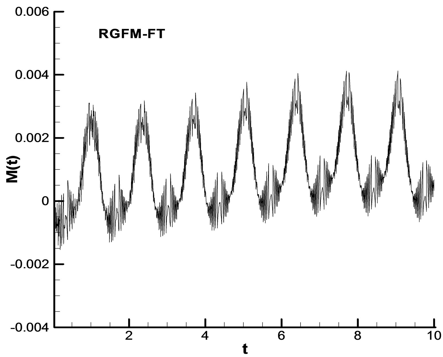 (b)
(b)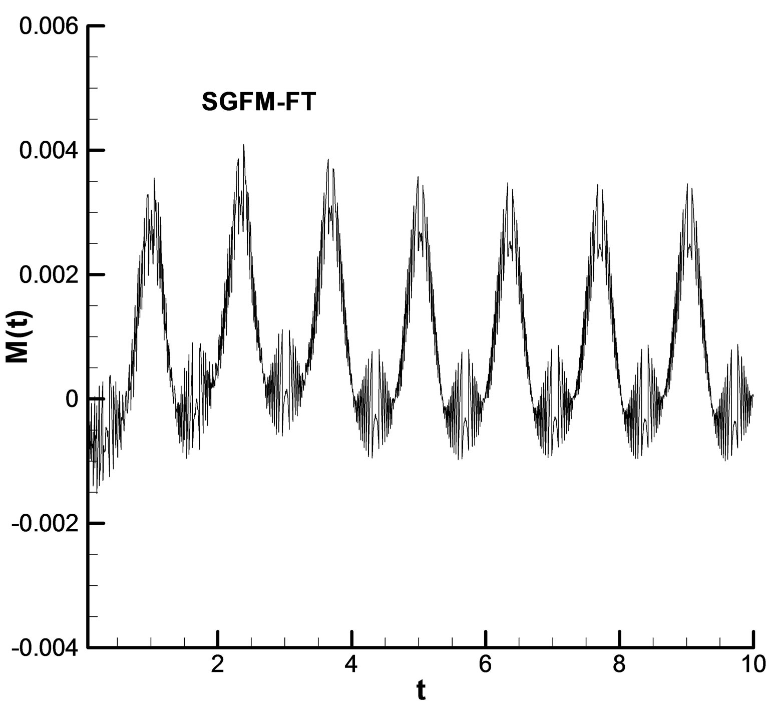 (c)
(c)
Figure 4. Comparison of conservation errors among the MGFM, the RGFM and the SGFM for Case 2 in Section 6. (a) the MGFM-FT and the SGFM-FT; (b) the RGFM-FT; (c) the SGFM-FT.
compared to RGFM. Figures 4(b) and (c) show that RGFM and SGFM have the same time evolution of the conservation errors.
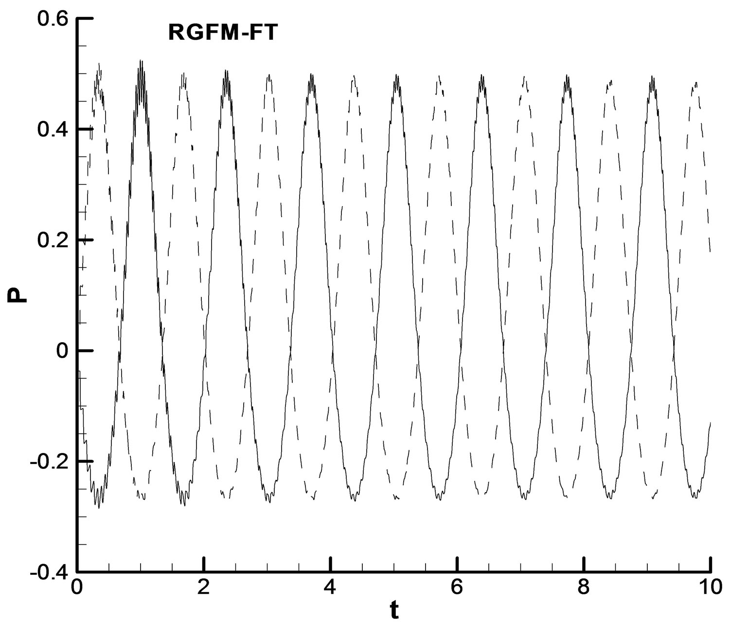
The wall pressure coefficients are given as
 (21)
(21)
 (22)
(22)
Figure 5 shows the time evolution of the pressure coef-
 (a)
(a)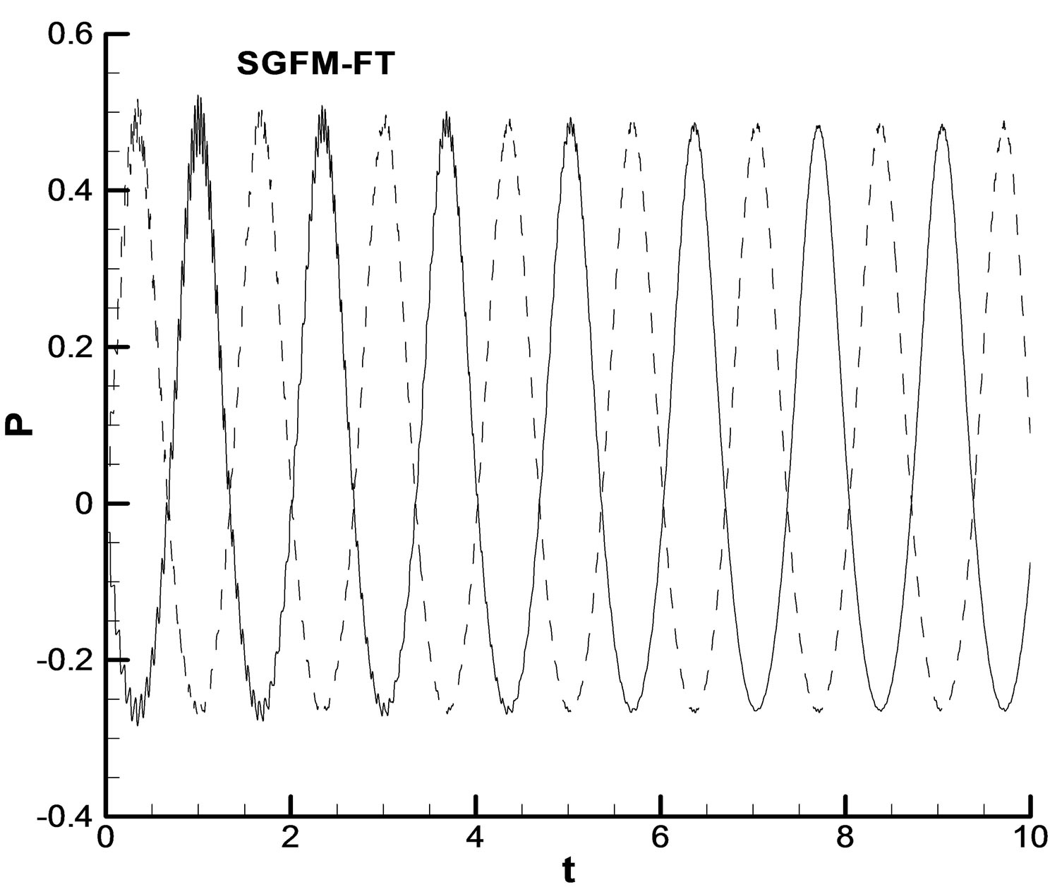 (b)
(b)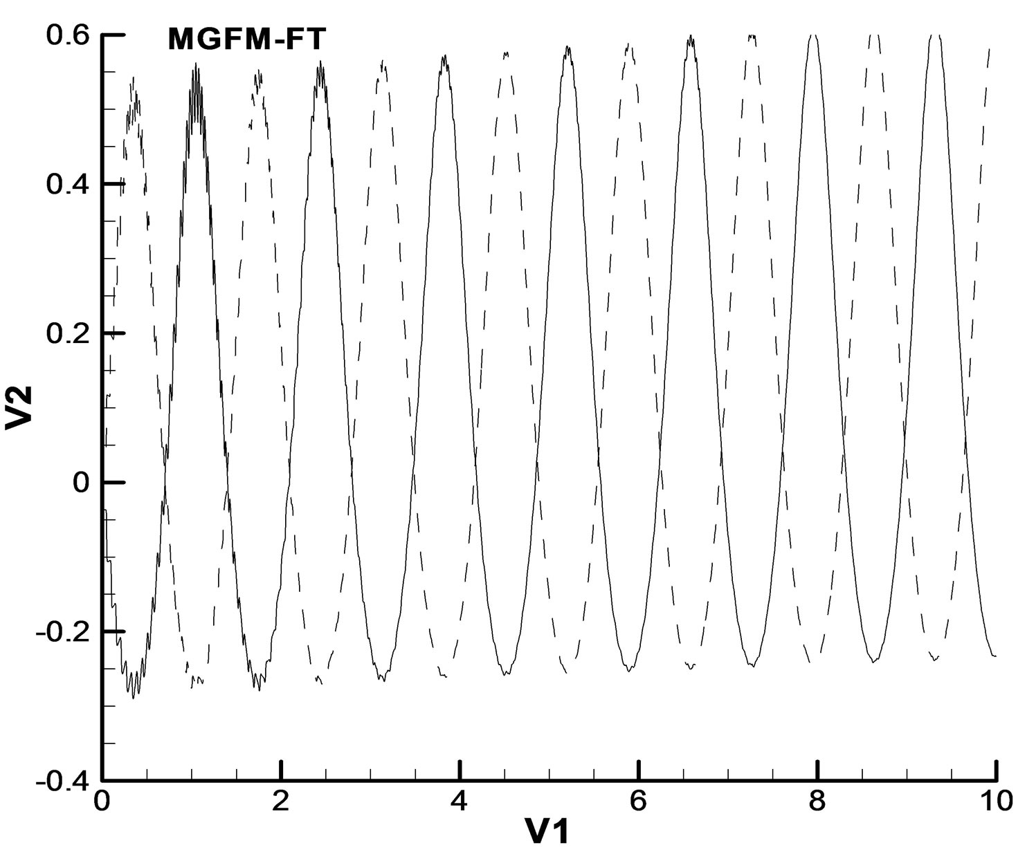 (c)
(c)
Figure 5. Time evolution of the pressure coefficients at boundaries for Case 2 in Section 6. Solid line: at the left boundary; dashed line: at the right boundary.
ficients at the wall boundaries calculated using MGFM, RGFM and SGFM. Figure 5(c) shows that there is a increase of the pressure amplitude with time for MGFM, while the pressure amplitude with RGFM and SGFM is changeless on the whole as show in Figures 5(a) and (b).
7. Applications
For all the one-dimensional problems the computational domain is taken as [0,1] with 201 nodes uniformly distributed unless stated otherwise.
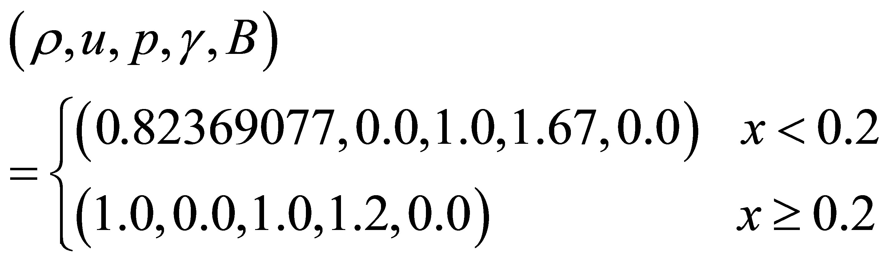
Problem 1: Gaseous shock in impedance-matching medium [8]. In this case a strong shock on the left side of the interface impacts on a gas-gas interface; The shock strength is 100 and the initial position of the shock is same as the interface, which is located at x0 = 0.2. The states on the left and right sides of the interface are defined respectively as
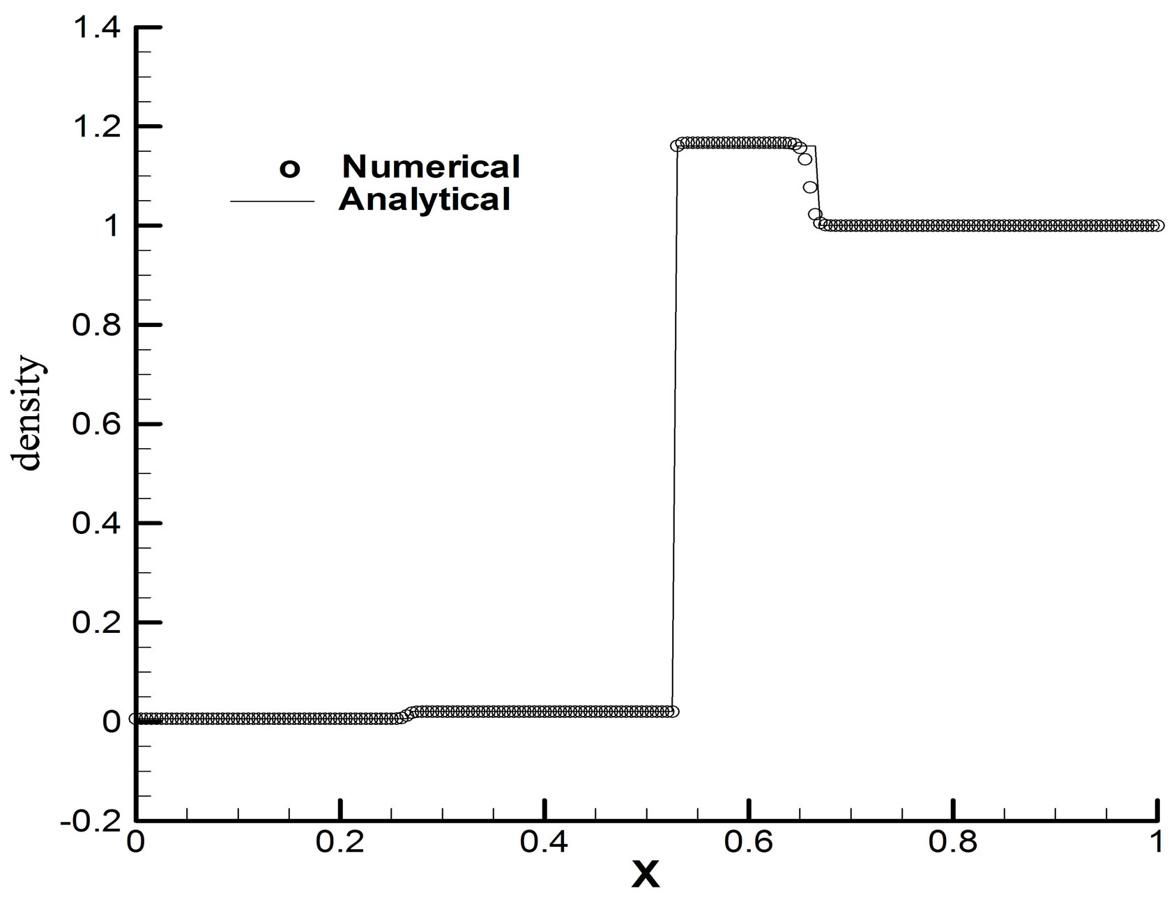
This problem is solved at time . The shock limiter is used [11]. Figures 6(a)-(c) show that the density, velocity and pressure obtained by the MUSCLbased SGFM-FT method compare to the analytical solution at time 0.06.
Problem 2: Strong shock impacting on a gas-water interface. A shock is located at the same position as the interface, which is initially located at . The strength of the incident gas shock is 1000. The states on the left and right sides of the interface are defined respectively as
For this case, a very strong shock is physically reflected back into the air. Figures 7(a)-(c) show that the density, velocity and pressure obtained by the MUSCLbased SGFM-FT method compare to the analytical solution at time 0.0007.
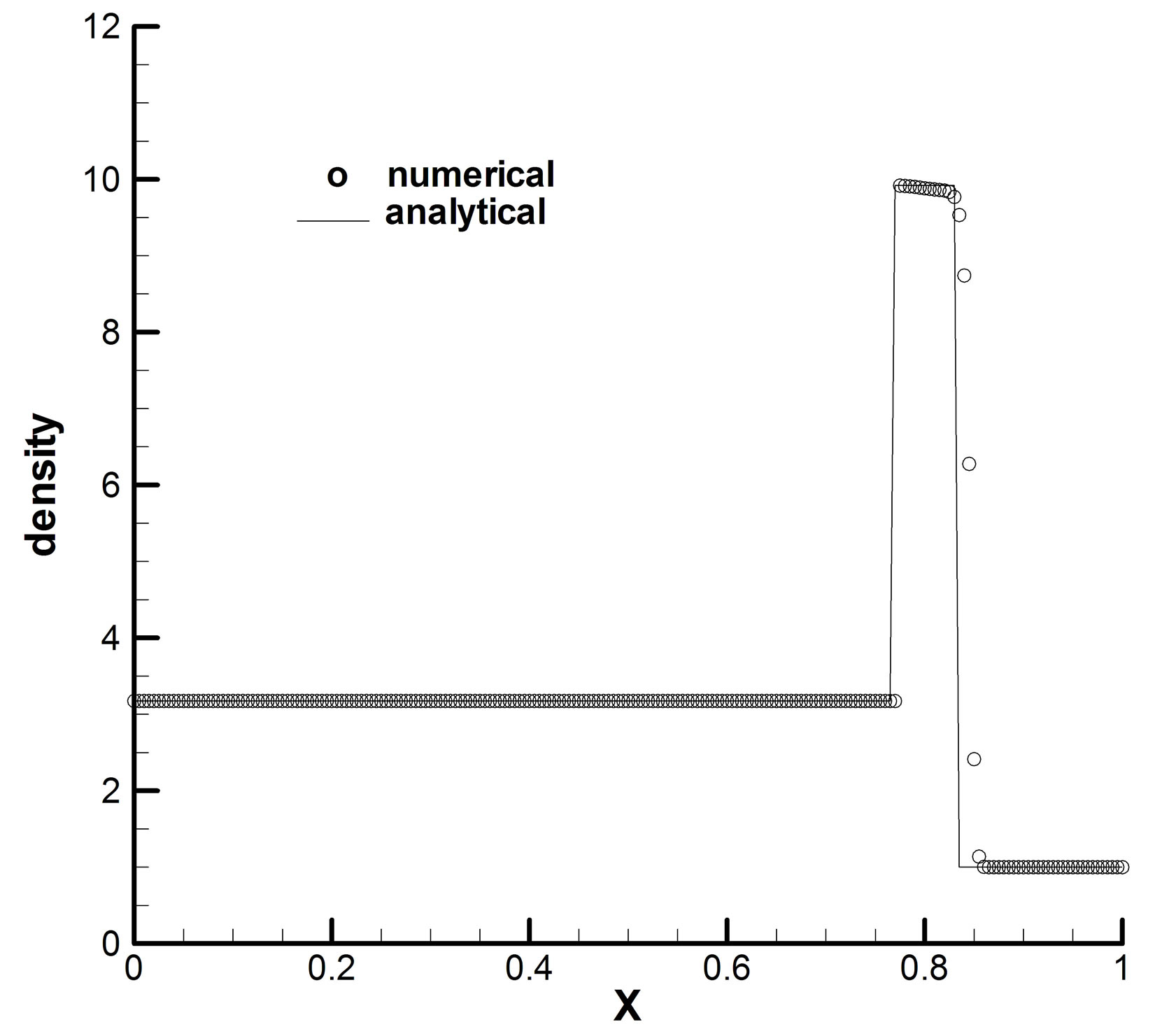
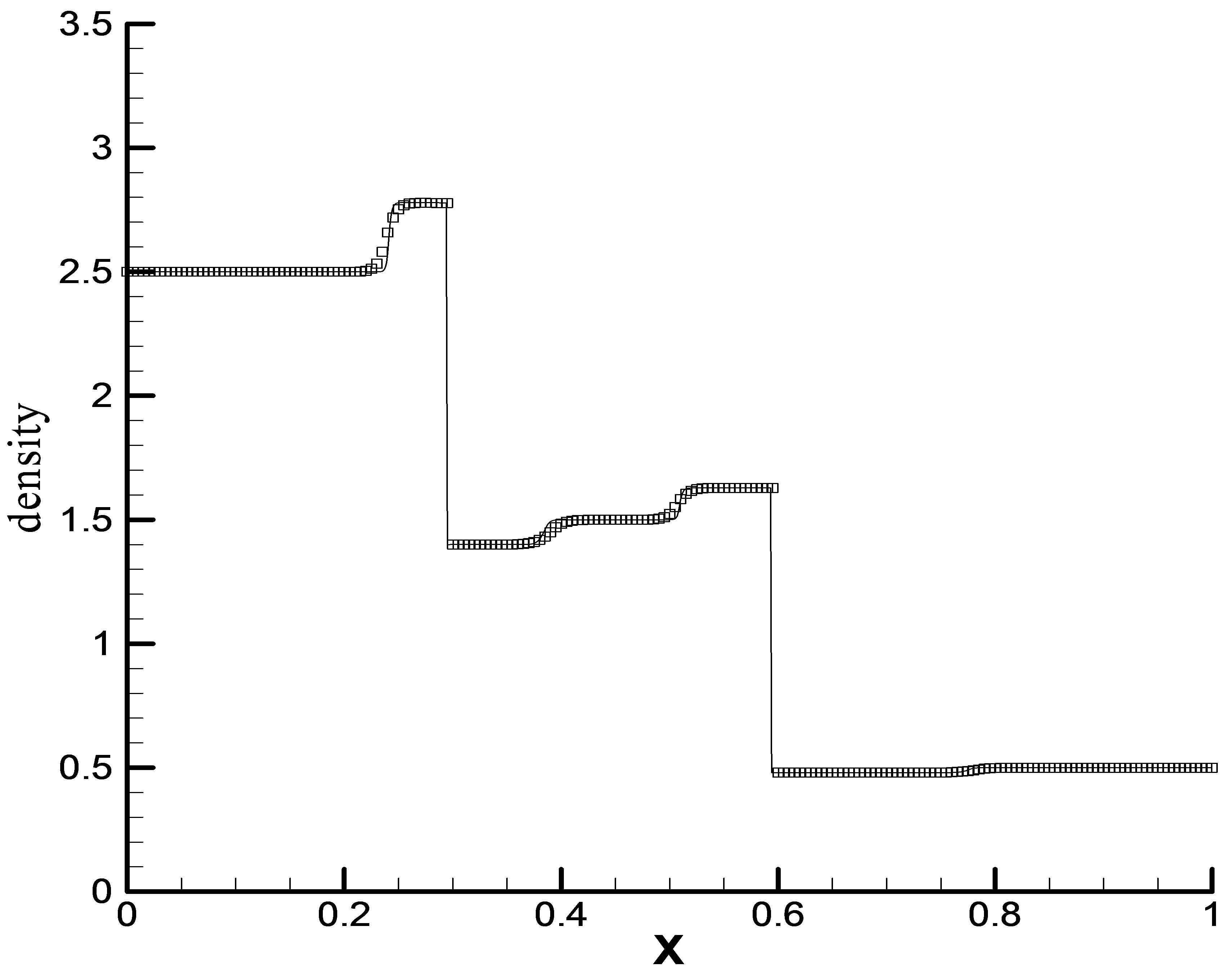
Problem 3: we solve the numerical example
This test has solution consisting of a rarefaction wave, two contact discontinuities and three shock waves. The
 (a)
(a)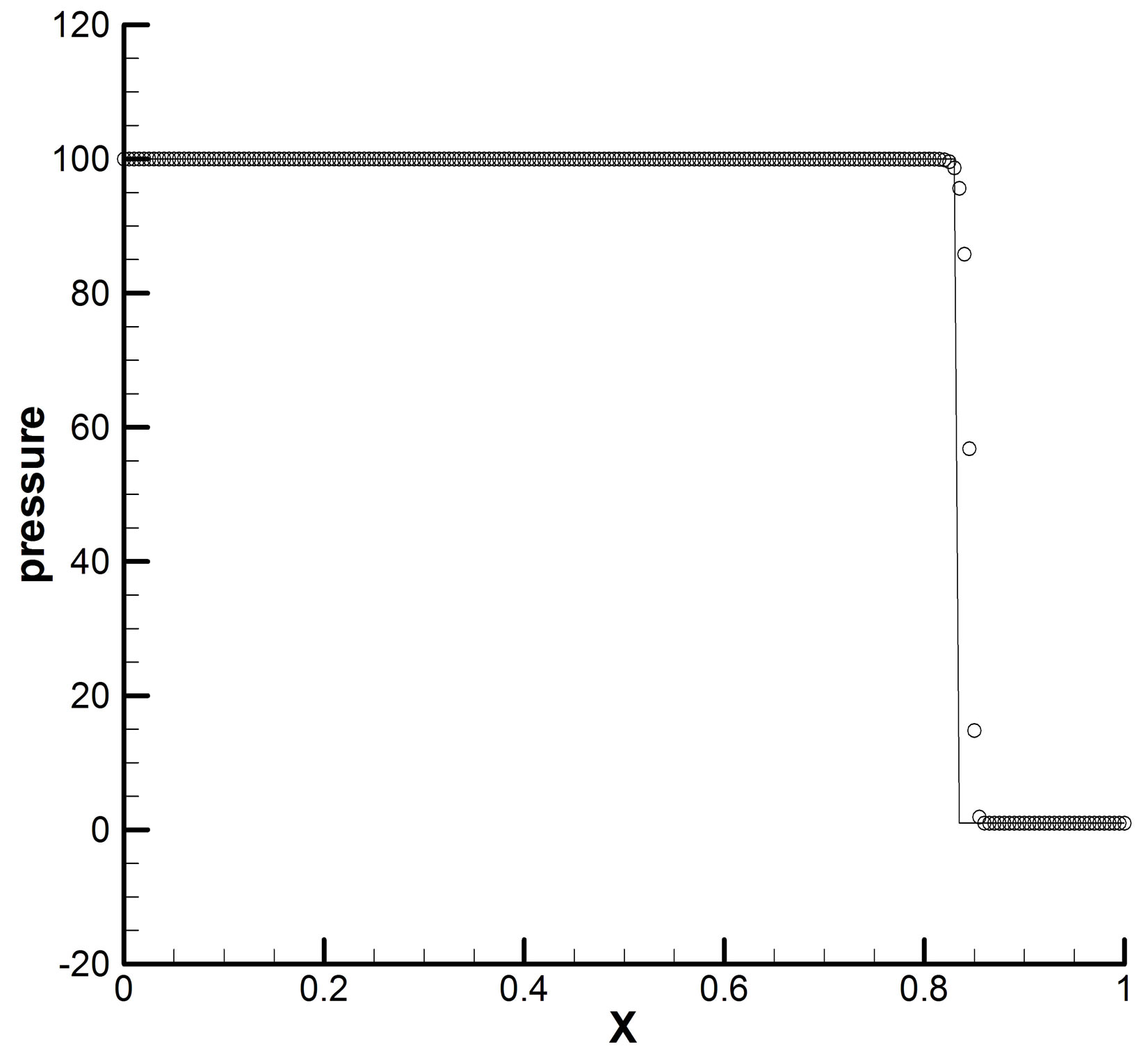 (b)
(b)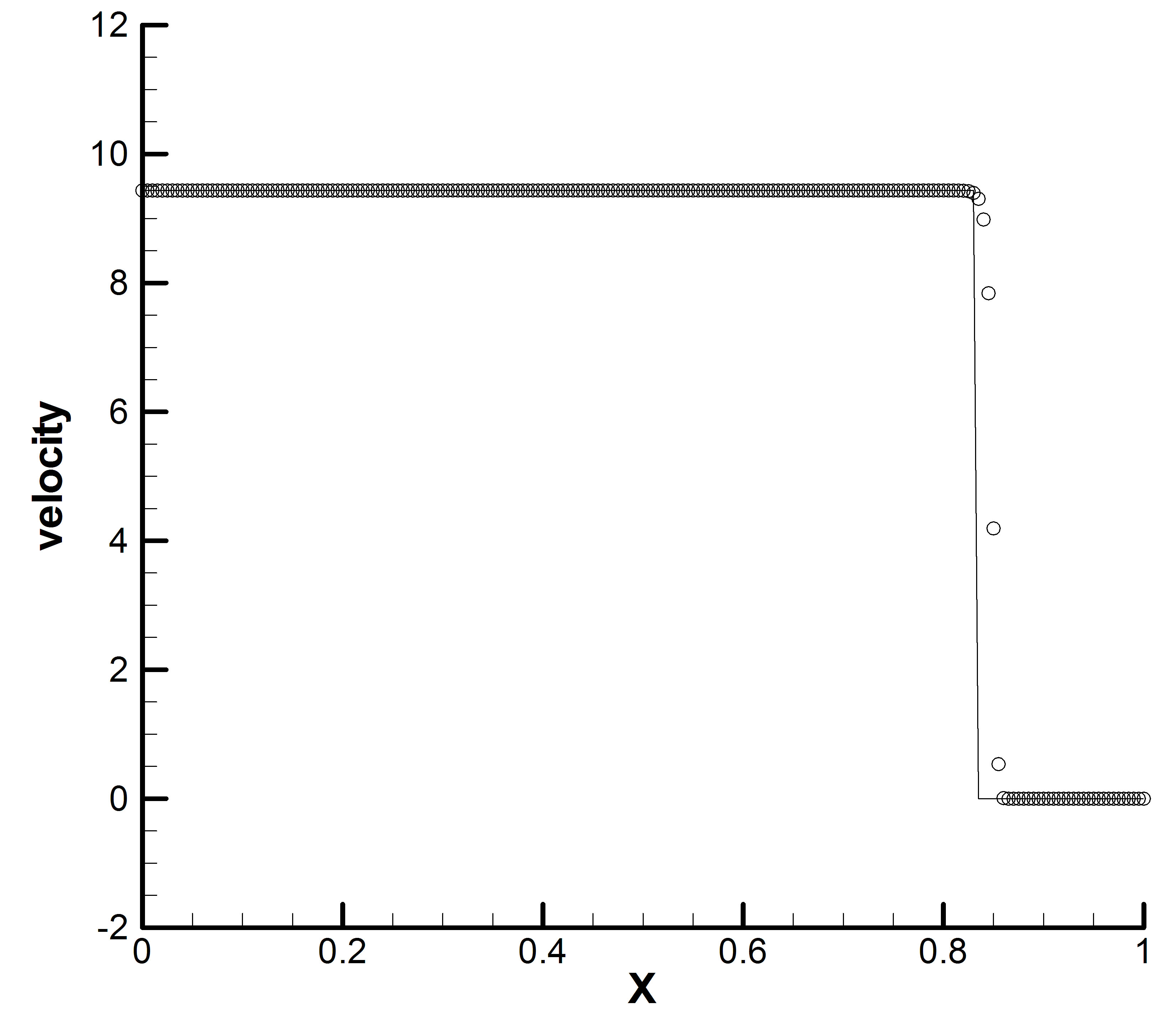 (c)
(c)
Figure 6. Problem 1.
MUSCL-based SGFM-FT method is used. Figures 8(a)- (c) describe the surprisingly good solution profiles at time 0.00028.
 (a)
(a)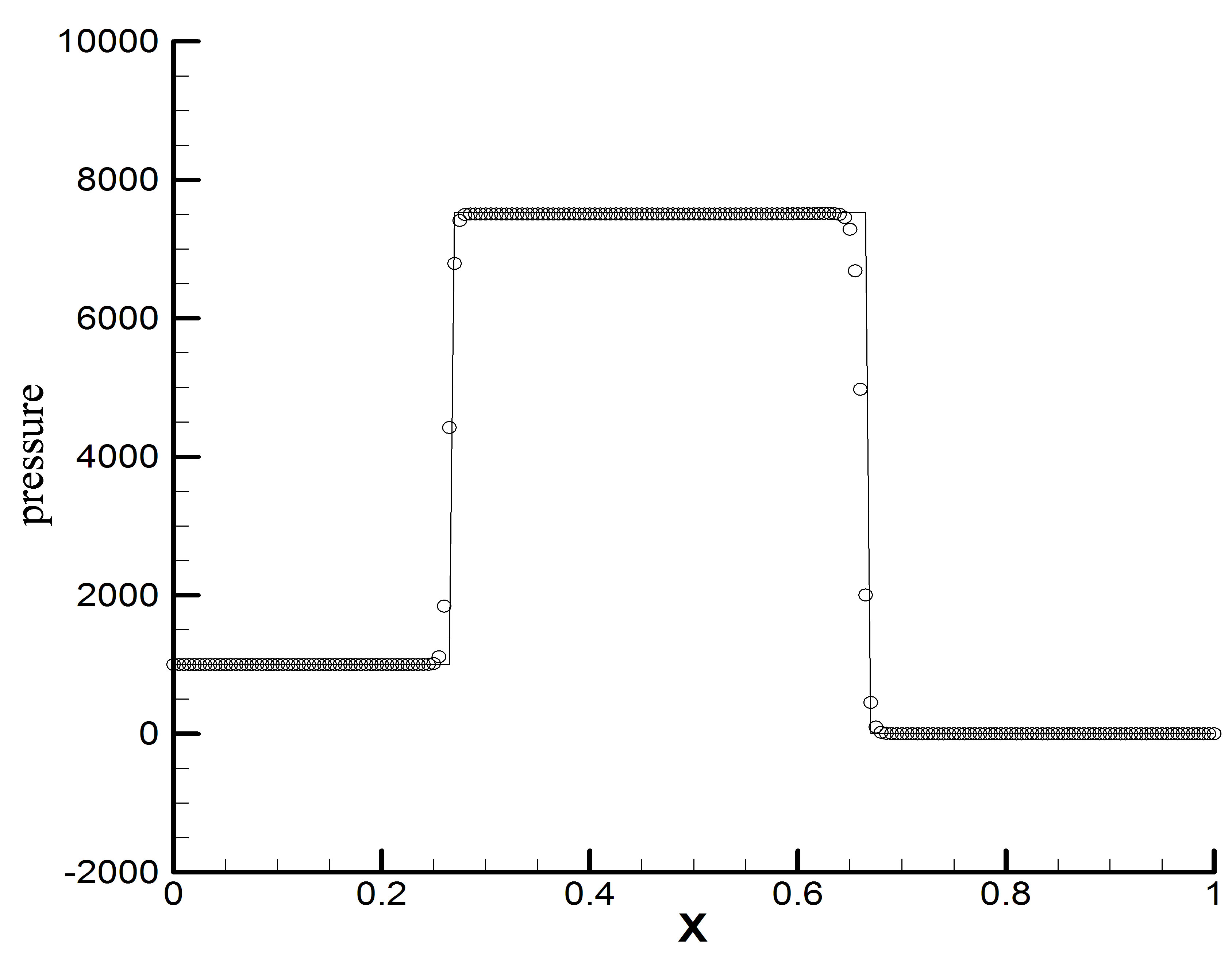 (b)
(b)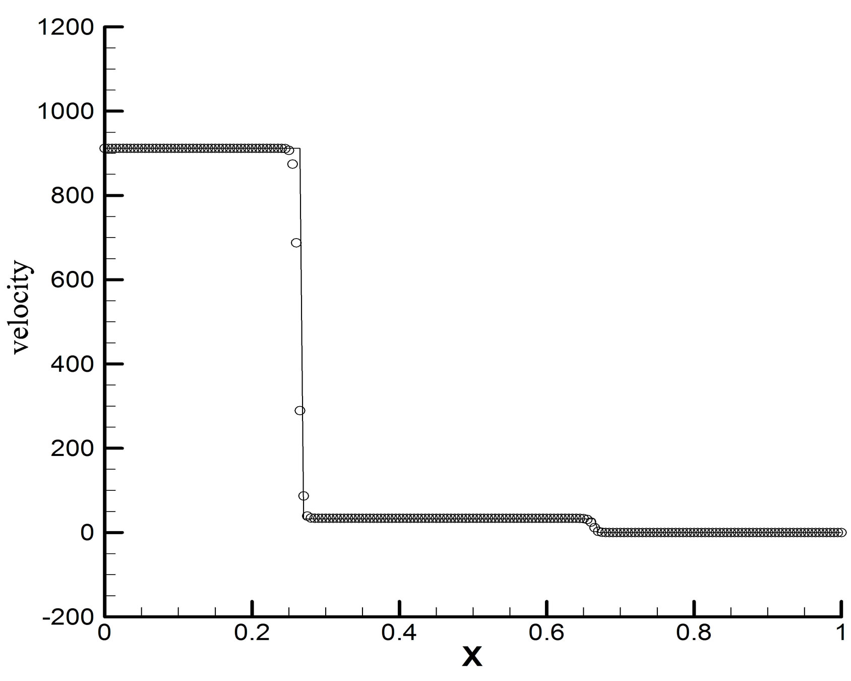 (c)
(c)
Figure 7. Problem 2.
8. Conclusion
In this paper, we developed a kind of GFM based on Riemann solutions. The RGFM is one of this type of GFM. A simplified front tracking algorithm had been used to track contact discontinuity. It is noted that different isentropic entropy can produce little effect on the conservation error and this kind of GFM has the property of reduced conservation error. A rigorous analysis is car-
 (a)
(a)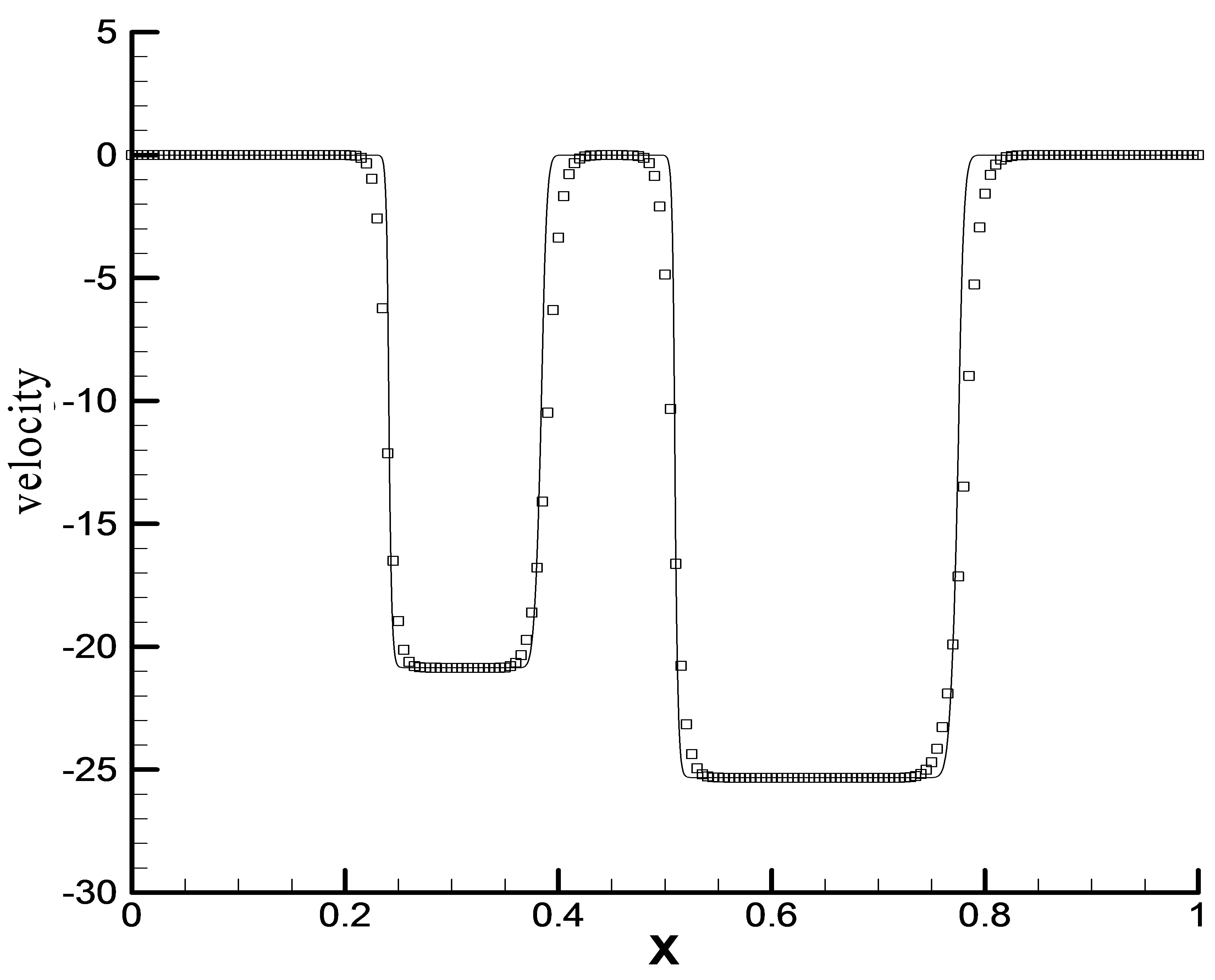 (b)
(b)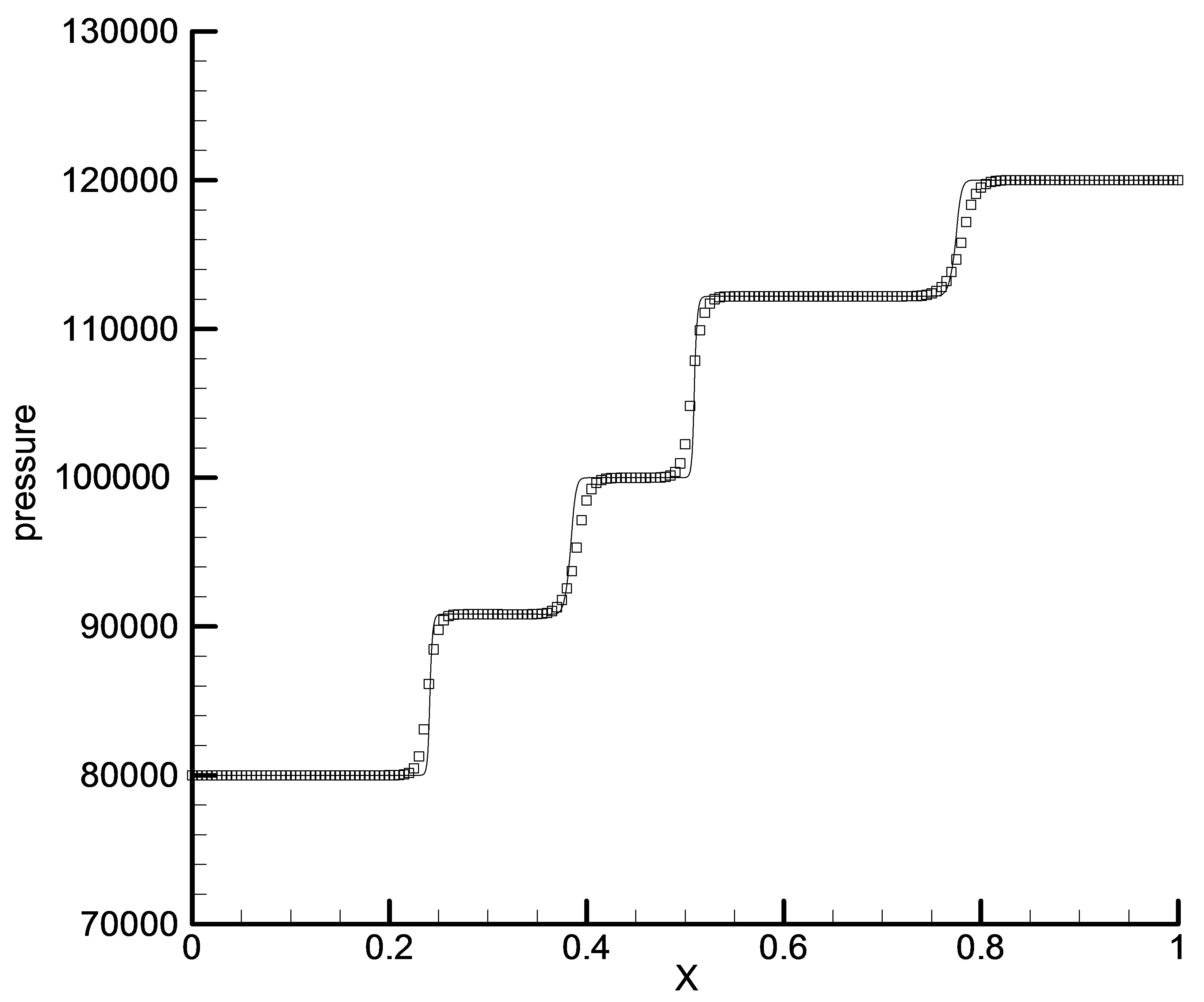 (c)
(c)
Figure 8. Problem 3: The “o” denotes the numerical results. The solid line denotes the exact solution.
ried out on the accuracy of the GFM when applied to the gas-gas Riemann problem. It is shown that at the material interface this type of GFM solution approximates the exact solution to at least second-order accuracy in the sense of comparing to the exact solution of a Riemann problem. When the shock monitor is used, discernible non-physical hump and trough which can not be avoided in shock impedance matching (-like) problems [7,8] do not appear for our proposed method. The ghost cell technique can be used for simulating compressible multimedium flow.
9. Acknowledgements
The researched work was supported by the National Natural Science Foundation of China (NO.91130030 and NO.11271188) and NUAA Research Funding (NO. NP2011033).
REFERENCES
- C. Hirt and B. Nichols, “Volume of fluid (VOF) Method for the Dynamics of Free Boundaries,” Journal of Computational Physics, Vol. 39, No. 1, 1981, pp. 201-225. doi:10.1016/0021-9991(81)90145-5
- D. Adalsteinsson and J. A. Sethian, “A Fast Level Set Method for Propagating Interfaces,” Journal of Computational Physics, Vol. 118, 1995, pp. 269-277. doi:10.1006/jcph.1995.1098
- H. Terashima and G. Tryggvason, “A Front-Tracking/ Ghost-Fluid Method for Fluid Interfaces in Compressible Flows,” Journal of Computational Physics, Vol. 228, No. 11, 2009, pp. 4012- 4037. doi:10.1016/j.jcp.2009.02.023
- R. P. Fedkiw, T. Aslam, B. Merriman and S. Osher, “A Non-Oscillatory Eulerian Approach to Interfaces in Multimaterial Flows (the Ghost Fluid Method),” Journal of Computational Physics, Vol. 152, No. 2, 1999, pp. 457- 492. doi:10.1006/jcph.1999.6236
- T. G. Liu, B. C. Khoo and K. S. Yeo, “Ghost Fluid Method for Strong Shock Impacting on Material Interface,” Journal of Computational Physics, Vol. 190, No. 2, 2003, pp. 651-681. doi:10.1016/S0021-9991(03)00301-2
- X. Y. Hu and B. C. Khoo, “An Interface Interaction Method for Compressible Multifluids,” Journal of Computational Physics, Vol. 198, No. 1, 2004, pp. 35-64. doi:10.1016/j.jcp.2003.12.018
- T. G. Liu, B. C. Khoo and C. W. Wang, “The Ghost Fluid Method for Compressible Gas-Water Simulation,” Journal of Computational Physics, Vol. 204, No. 1, 2005, pp. 193-221. doi:10.1016/j.jcp.2004.10.012
- C. W. Wang, T. G. Liu and B. C. Khoo, “A Real Ghost Fluid Method for the Simulation of Multimedium Compressible Flow,” Journal on Scientific Computing, Vol. 28, No. 1, 2006, pp. 278-302.
- Y. Hao and A. Prosperetti, “A Numerical Method for Three-Dimensional Gas-Liquid Flow Computations,” Journal of Computational Physics, Vol. 196, No. 1, 2004, pp. 126-144. doi:10.1016/j.jcp.2003.10.032
- G. Tryggvason, B. Bunner, A. Esmaeeli, D. Juric, N. A. Rawahi, W. Tauber, J. Han, S. Nas and Y. J. Jan, “A Front Tracking Method for the Computations of Multiphase Flow,” Journal of Computational Physics, Vol. 169, No. 2, 2001, pp. 708-759. doi:10.1006/jcph.2001.6726
- D. H.Wang, N. Zhao, O. Hu and J. M. Lui, “A Ghost Fluid Based Front Tracking Method for Multimedium Compressible Flows,” Acta Mathematica Sinica, Vol. 29B, No. 6, 2009, pp. 1629-1646.
- J. Glimm, J. Grove, X. L. Li and N. Zhao, “Simple Front Tracking,” Contemporary Mathematics, Vol. 238, 1999, pp. 133-149. doi:10.1090/conm/238/03544
- T. G. Liu and B. C. Khoo, “The Accuracy of the Modified Ghost Fluid Method for Gas-Gas Riemann Problem,” Applied Numerical Mathematics, Vol. 57, No. 5-7, 2007, pp. 721-733.