Open Journal of Fluid Dynamics
Vol.2 No.4(2012), Article ID:25499,4 pages DOI:10.4236/ojfd.2012.24013
Computing the Pressure Drop of Nanofluid Turbulent Flows in a Pipe Using an Artificial Neural Network Model
1Department of Mechanical Engineering, Faculty of Engineering, Taif University, Al-Hawiah, Saudi Arabia
2Mechanical Engineering Department, Faculty of Engineering, Assiut University, Assiut, Egypt
3Mechanical Power Engineering Department, Faculty of Engineering, Mansoura University, Mansoura, Egypt
Email: youssef2056@yahoo.com
Received October 8, 2012; revised November 12, 2012; accepted November 21, 2012
Keywords: Artificial Neural Networks (ANNs); Turbulent Flow; Nanofluids; Pressure Drop
ABSTRACT
In this study, an Artificial Neural Network (ANN) model to predict the pressure drop of turbulent flow of titanium dioxide-water (TiO2-water) is presented. Experimental measurements of TiO2-water under fully developed turbulent flow regime in pipe with different particle volumetric concentrations, nanoparticle diameters, nanofluid temperatures and Reynolds numbers have been used to construct the proposed ANN model. The ANN model was then tested by comparing the predicted results with the measured values at different experimental conditions. The predicted values of pressure drop agreed almost completely with the measured values.
1. Introduction
Many industrial processes involve the transfer of heat by means of a flowing fluid in either the laminar or turbulent regime as well as flowing or stagnant boiling fluids. Most of these processes would benefit from a decrease in the flow resistance of the heat-transfer fluid resulting in smaller heat-transfer systems with lower capital cost and improved thermal efficiencies. Nanofluid is the name conceived by the Argonne National Laboratory (ANL) to describe a fluid in which nanometer-sized solid particles, fibers, or tubes are suspended in liquids such as water, engine oil, or ethylene glycol (EG). Nanofluids have the potential to reduce thermal resistances and can be used in different industrial manufacturing applications of electronics and in transportation, medical, and food industries [1].
While thermal properties are important for heat transfer applications, the viscosity is also important in designing nanofluids for flow and heat transfer applications because the pressure drop and the resulting pumping power depend on the viscosity. Many experimental investigations on the heat transfer performance and pressure drop of different nanofluids with various nanoparticle volume-concentrations in both laminar and turbulent flow regimes have been reported [2-8]. These experimental results showed different trends in the variations of the pressure drop values of the nanofluids. So far, the results of Duangthongsuk and Wongwises [2] showed that the pressure drop with nanofluids was slightly higher than with the base fluid and increases with increasing the volume concentrations. Also, the results of Duangthongsuk and Wongwises [3] and He et al. [4] disclosed that the pressure drop with nanofluids was very close to that of the base fluid. Teng et al. [5] reported that the value of pressure drop enhancement for titanium dioxide (TiO2) nanofluid in a circular pipe is lower under turbulence but higher under laminar flow conditions. Recently, turbulent heat transfer behavior of TiO2 nanofluid in a circular pipe under fully-developed turbulent regime for various volumetric concentrations was investigated experimenttally by Sajadi and Kazemi [6]. Their measurements showed that the pressure drop of nanofluid was slightly higher than that of the base fluid and increased with increasing the volume concentration. While, the results of Fotukian and Esfahany [7] indicated that the maximum increase in pressure drop was about 20% for nanofluid, Vajjha et al. [8] reported that the pressure loss of nanofluids increases with an increase in particle volumeconcentrations and the increase of pressure loss for a 10% Al2O3 nanofluid was about 4.7 times than that of the base fluid.
Various theoretical/numerical models were proposed to study the mechanism and predict the thermal conductivity and pressure drop of different nanofluids [9-11]. The numerical studies of nanofluids can be conducted using single-phase (homogenous) or two-phase approaches. In the former approach it is assumed that the fluid phase and nanoparticles are in thermal equilibrium with zero relative velocity. While, in the latter approach, base fluid and nanoparticles are considered as two different liquid and solid phases with different momentums respectively [9]. Some of the published articles were related to the investigation of laminar convective heat transfer of nanofluids [9,10], while, the others were concerned with turbulent ones [11]. Fard et al. [9] used a Computational Fluid Dynamics (CFD) approach regarding single-phase and two-phase models to study laminar convective heat transfer of nanofluids with different volume concentrations in a circular tube. Their numerical results have clearly shown that nanofluids with higher volume-concentration have higher pressure drop and two-phase model showed better agreement with experimental data. The commercial CFD package, FLUENT, was used by Demir et al. [10] for solving the volumeaveraged continuity, momentum, and energy equations of different nanofluids flowing in a horizontal tube under constant temperature condition. Their numerical results have indicated that pressure drop increases with increasing the particle loading parameter and Reynolds number because of increasing velocity and viscosity of nanofluid. Turbulent flow and heat transfer of three different nanofluids flowing through a circular tube under constant heat flux condition have been numerically analyzed by Namburu et al. [11]. They assumed and used singlephase fluid model to solve two-dimensional steady, forced turbulent convection flow of nanofluid flowing inside a straight circular tube. Two-equation turbulence model of launder and Spalding was adopted by Namburu et al. [11] in their numerical analysis. Their computed results indicated that pressure loss increases with increase in the volume concentration of nanofluids.
Based on the preceding literature on both experimental and theoretical reviews, one could conclude that the variations in the experimental data of the pressure drop of nanofluids are attributed to the difficulties of the experimental studies. These difficulties are mainly due to lack in understanding the details and mechanisms of heat transfer phenomenon that increase the thermal conductivity and pressure drop in nanofluids [12]. On the other side, the algorithms employed in numerical studies particularly with turbulent flows are usually complicated since involving the solution of complex differential equations. As a corollary, these programs usually require large computer power and need a considerable amount of time to give accurate predictions. Instead of carrying experimental measurements or using complex algorithms and mathematical routines in classical methods to calculate the pressure drop in a pipe under turbulent regime, a simpler model is needed alternative of CFD tools for preliminary simulations under well known conditions and usual ranges of the main flow parameters.
The objective of this study is to develop an Artificial Neural Network (ANN) model to calculate the pressure drop values of nanofluid at different particle volumetricconcentrations, nanoparticle diameters, nanofluid temperatures and different values of Reynolds number. Titanium dioxide dispersed in water (TiO2-water) was selected as a nanofluid to assess the proposed ANN model due to experimental data are available in the literature.
2. ANN Model
2.1. ANN Model Structure
Artificial neural networks (ANNs) are computational model constructed of many simple interconnected elements called neurons, which are based on the information processing system of the human brain Figure 1 shows the architecture of the neural network model used in this work. The basic structure is a multilayer ANN model where the chosen four inputs are fed into the first layer of hidden units. There, the circles represent the neurons (weights, bias, and activation functions) and the lines represent the connections between the inputs and neurons, and between the neurons in one layer and those in the next layer. Several studies have found that a three-layered neural network, where there are three stages of neural processing between the inputs and outputs, can approximate any nonlinear function to any desired accuracy [13-15]. Each layer consists of units which receive their input from units from a layer directly below and send their output to units in a layer directly above the unit. Each connection to a neuron has an adjustable weighting factor associated with it. The output of the hidden units is distributed over the next layer of hidden units, until the last layer of hidden units, of which the outputs are fed into a layer of no output units. Training of the ANN model typically implies adjustments of connection weights and biases so that the differences between ANN outputs and desired outputs are minimized.
2.2. Back-Propagation Training Algorithm
Back-propagation training, used in this investigation, is one of the most popular ANN training methods. The basic back-propagation algorithm adjusts the weights in the steepest descent direction (negative of the gradient). This is the direction in which the error decreases most rapidly. To explain the back-propagation rule in detail, the three-layer network shown in Figure 1 will be used. The training phase is divided into two phases as follows:
1) Forward-propagation phase: In the first phase,

Figure 1. A schematic of neural network model.
input data are sent from the input layer to the output layer, i.e.,  is propagating from the input layer to the output layer Y.
 (1)
(1)
 (2)
(2)
where Zq, Yi are data sets for hidden layers and ANN model output, respectively, Wiq and Vqj represent weights in the hidden-to-output and input-to-hidden connections, respectively, f is the activation function .
2) Back-propagation phase: In the second phase, the errors between target outputs, Y, and predicted outputs, d, are calculated and propagated backwardly to the input layer in order to change the weights of hidden layers by using the gradient descent method.
The algorithm tries to minimize the objective function, i.e. the least square error between the predicted and the target outputs, which is given by:
 (3)
(3)
where p represents the number of training datasets and o represents the number of output nodes. Then the algorithm uses the steepest-descent direction to adjust the weights in the hidden-to-output and input-to-hidden connections and as follows:
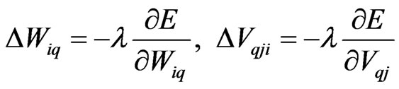 (4)
(4)
where λ is the learning rate.
Since this algorithm requires a learning rate parameter to determine the extent to which the weights change during iteration, i.e., the step sizes, its performance depends on the choice of the value of the learning rate. The two phases are iterated until the performance error decreased to certain small range [13-15].
2.3. Activation Functions
Activation functions are used in ANNs to produce continuous values rather than discrete ones. The activation functions used in hidden layer neurons are tan sigmoid functions and the piecewise linear activation function is used for the last layer neurons. The logistic activation function or more popularly referred to as the sigmoid function is semi-linear in character, differentiable and produces a value between 0 and 1. The mathematical expression of this sigmoid function is:
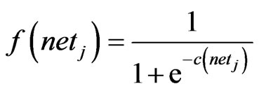 (5)
(5)
where c is a constant which controls the firing angle of the sigmoid. When c is large, the sigmoid becomes like a threshold function and when is c small, the sigmoid becomes more like a straight line (linear). When c is large learning is much faster but a lot of information is lost, however when c is small, learning is very slow but information is retained. Because this function is differentiable, it enables the back-propagation algorithm to adapt the lower layers of weights in a multilayer neural network.
3. ANN Model Training
The present study, the effects of four independent quantities on the pressure drops of Titanium dioxide dispersed in water (TiO2-water) flowing through a pipe under turbulent flow regime is investigated. These four independent quantities are the particle volumetric concentration in nanofluid, temperature of nanofluid, nanoparticle diameter, and Reynolds number of flow. Therefore, the values of these four inputs are fed into the hidden layer. Each connection to a neuron has adjustable weighting factor associated with it. The outputs of the hidden layer are fed into a layer of one output units which is the pressure drop DP of nanofluid. The activation functions in hidden layer neurons are tan sigmoid functions and the piecewise linear activation function is used for the last layer neurons. The algorithm tries to minimize the objective function, i.e. the least square error between the predicted and the target outputs. Several neural network models were trained with various design including number of hidden layers and number of nodes in each hidden layer. The selection of the optimum model was based on minimizing the difference between the neural network results and the desired output. It was found that, best structure of the ANN model has an input layer, a hidden layer and an output layer. Therefore, the developed ANN architecture has a configuration as shown in Figure 1. The input layer comprises all of the four input variables, which are connected to neurons in the hidden layer through the weights assigned for each link. The number of neurons in the hidden layer is found by optimizing the network. All the four input parameters and their range of values of Titanium dioxide dispersed in water (TiO2-water) used to develop the neural network model are mentioned in Table 1 [2-4].
The developed ANN model was trained using some of the experimental data of TiO2-water. The experimental data set consists of 106 values. These were divided into two groups, of which the 90 values were used for training/learning of the ANN model. This means that the experimental data of Duangthongsuk and Wongwises [2], the experimental data of Duangthongsuk and Wongwises [3] at 20˚C and 25˚C, as well as the experimental data of He et al. [4] were used for training of the proposed model. On the other hand, 16 values of the experimental
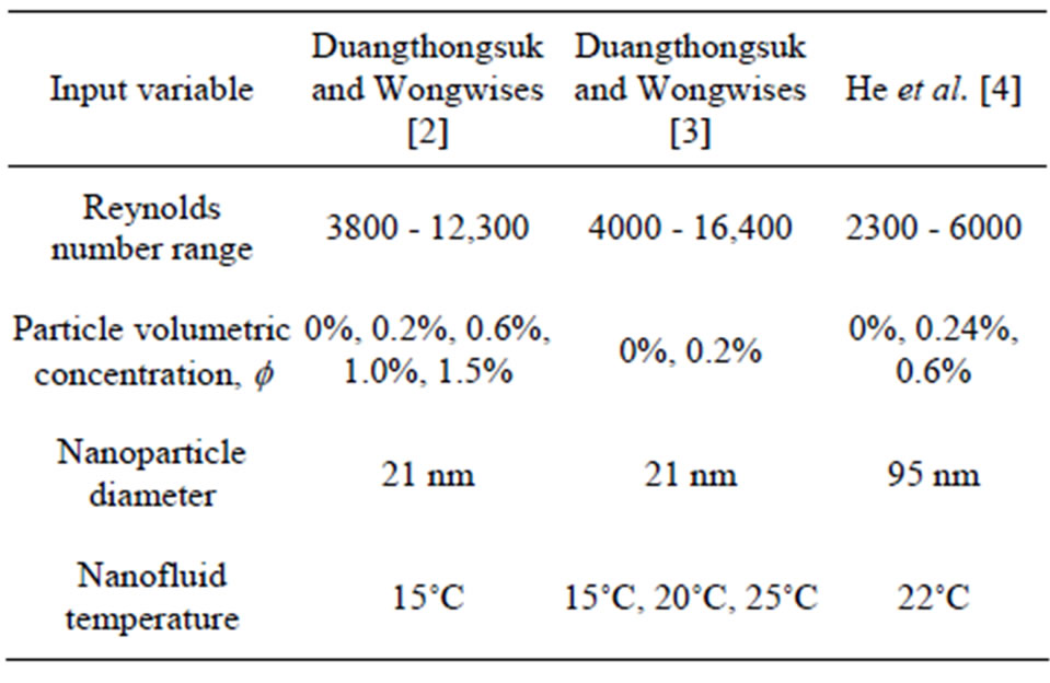
Table 1. The range of input parameters used in training and testing the proposed ANN model [2].
data of Duangthongsuk and Wongwises [3] at 15˚C of nanofluid temperature were chosen to validate the proposed ANN model.
Figure 2 shows the distribution of the ANN predicted pressure drop DP for 21 nm nanoparticle at 15˚C temperature of TiO2 along with the experimental measured values of Duangthongsuk and Wongwises [2] at the same conditions. Excellent agreement is found between the trained values of the model and both the experimental measurements of Duangthongsuk and Wongwises [2]. Variations of the ANN predicted pressure drop versus the Reynolds number for 21 nm nanoparticle at 20˚C and 25˚C nanofluid temperatures as well as for 95 nm nanoparticle at 22˚C nanofluid temperature are shown in Figures 3 and 4, respectively. Also, included in these figures are the experimental measurements of Duangthongsuk and Wongwises [3] and He et al. [4]. It can be seen in these figures that the trained values are in excellent agreement with the experimentally ones. It can be ultimately concluded that the proposed ANN model behaves excellently in the training stage and, therefore, it’s expected to exhibit a satisfactory performance in the validation stage as can be seen in the next section.
4. Results of Validation
A set of experimental data (16 values) of Duangthongsuk and Wongwises [3] for 21 nm nanoparticle of TiO2 dispersed in water at 15˚C nanofluid temperature was used to validate the proposed ANN model. In Figure 5, the predicted results of pressure drop, DP, from the ANN model are compared to the experimental measured data
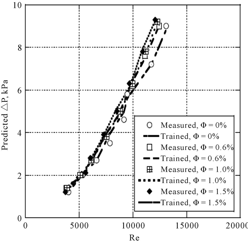
Figure 2. Comparison of ANN-predicted values of pressure drop DP with Reynolds number Re for the training data set for 21 mm nanoparticle at 15˚C nanofluid temperature.
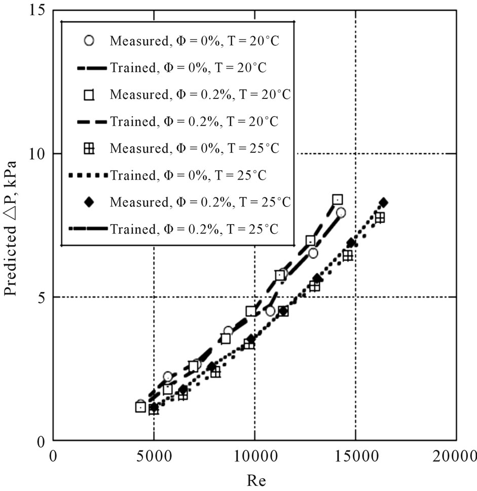
Figure 3. Comparison of ANN-predicted values of pressure drop DP with Reynolds number Re for the training data set for 21 nm nanoparticle at 20˚C and 25˚C nanofluid temperatures.
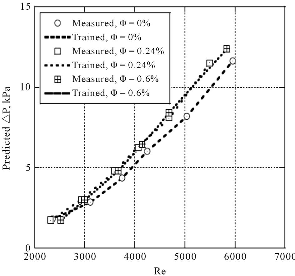
Figure 4. Comparison of ANN-predicted values of pressure drop DP with Reynolds number Re for the training data set for 95 nm nanoparticle at 22˚C nanofluid temperature.
of Duangthongsuk and Wongwises [3]. What has to be noticed from Figure 5 is that the predicted values of pressure drop are in excellent agreement with the experimental data of Duangthongsuk and Wongwises [3]. To evaluate the accuracy of the ANN model predictions, Figure 6 shows another prediction performance measurement which a straight line indicating the perfect prediction is provided. Note that in Figures 5 and 6, the
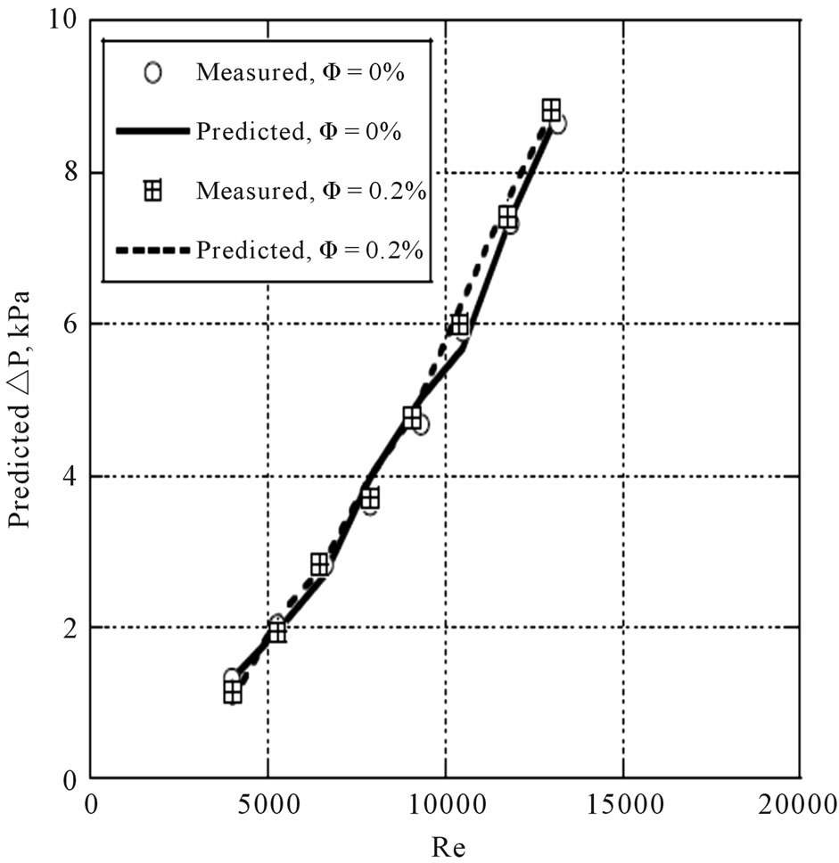
Figure 5. Comparison of ANN-predicted values of pressure drop DP with Reynolds number Re for the test data set for 21 nm nanoparticle at 15˚C nanofluid temperature.

Figure 6. Comparison of experimentally measured and ANN-predicted values of pressure drop DP for the test data set for 21 nm nanoparticle at 15˚C nanofluid temperature.
comparisons were made using the experimental values only from the test data set, which was not introduced to the ANN model during the training process as mentioned before and was selected randomly from experimentally obtained data set of Duangthongsuk and Wongwises [3]. It can be seen in Figure 6 that the predicted results of pressure drop mimics almost the corresponding experimental results.
5. Conclusion
An ANN model to predict the pressure drop of TiO2- water flowing through a pipe under different turbulent flow conditions has been proposed in this study. Different experimental measured data with different particle volumetric-concentrations, nanoparticle diameters, and nanofluid temperatures at different values of Reynolds number were used to construct the present ANN model. The ANN model based on a multilayer perception with back propagation learning algorithm was developed. Excellent agreement between the predicted values and the experimental data at different parameters for pressure drop of TiO2-water nanofluid was clearly noticed. More experimental measured data for other nanofluids are needed to widen the range of application of the proposed ANN model.
6. Acknowledgements
The financial support of the University of Taif, Saudi Arabia is highly acknowledged.
REFERENCES
- W. Yu, D. M. France, S. U. S. Choi and J. L. Routbort, “Review and Assessment of Nanofluid Technology for Transportation and Other Applications,” Energy Systems Division, Argonne National Laboratory, DuPage, 2007. doi:10.2172/919327
- W. Duangthongsuk and S. Wongwises, “An Experimental Study on the Heat Transfer and Pressure Drop of TiO2- Water Nanofluids Flowing under a Turbulent Regime,” International Journal of Heat and Mass Transfer, Vol. 53, No. 1-3, 2010, pp. 334-344. doi:10.1016/j.ijheatmasstransfer.2009.09.024
- W. Duangthongsuk and S. Wongwises, “Heat Transfer Enhancement and Pressure Drop Characteristics of TiO2-Water Nanofluid in a Double-Tube Counter Flow Heat Exchanger,” International Journal of Heat and Mass Transfer, Vol. 52, No. 7-8, 2009, pp. 2059-2067. doi:10.1016/j.ijheatmasstransfer.2008.10.023
- Y. He, Y. Jin, H. Chen, Y. Ding, D. Cang and H. Lu, “Heat Transfer and Flow Behavior of Aqueous Suspensions of TiO2 Nanoparticles (Nanofluids) Flowing Upward through a Vertical Pipe,” International Journal of Heat and Mass Transfer, Vol. 50, No. 11-12, 2007, pp. 2272-2281.
- T.-P. Teng, Y.-H. Hung, C.-S. Jwo, C.-C. Chen and L.-Y. Jeng, “Pressure Drop of TiO2 Nanofluid in Circular Pipes,” Particuology, Vol. 9, No. 5, 2011, pp. 486-491. doi:10.1016/j.partic.2011.05.001
- A. R Sajadi and M. H. Kazemi, “Investigation of Turbulent Convective Heat Transfer and Pressure Drop of TiO2/Water Nanofluid in Circular Tube,” International Communications in Heat and Mass Transfer, Vol. 38, No. 10, 2011, pp. 1474-1478. doi:10.1016/j.icheatmasstransfer.2011.07.007
- S. M. Fotukain and M. N. Esfahany, “Experimental Study of Turbulent Convective Heat Transfer and Pressure Drop of Dilute CuO/Water Nanofluid inside a Circular Tube,” International Communications in Heat and Mass Transfer, Vol. 37, No. 2, 2010, pp. 214-219. doi:10.1016/j.icheatmasstransfer.2009.10.003
- R. S. Vajjha, D. K. Das and D. P. Kulkarni, “Development of New Correlations for Convective Heat Transfer and Friction Factor in Turbulent Regime for Nanofluids,” International Journal of Heat and Mass Transfer, Vol. 53, No. 21-22, 2010, pp. 4607-4618. doi:10.1016/j.ijheatmasstransfer.2010.06.032
- M. H. Fard, M. N. Esfahany and M. R. Talaie, “Numerical Study of Convective Heat Transfer of Nanofluids in a Circular Tube Two-Phase Model versus Single-Phase Model,” International Communications in Heat and Mass Transfer, Vol. 37, No. 1, 2010, pp. 91-97. doi:10.1016/j.icheatmasstransfer.2009.08.003
- H. Demir, A., S. Dalkilic, N. A. Kürekci, W. Duangthongsuk and S. Wongwise, “Numerical Investigation on the Single Phase Forced Convection Heat Transfer Characteristics of TiO2 Nanofluids in a Double-Tube Counter Flow Heat Transfer,” International Communications in Heat and Mass Transfer, Vol. 38, No. 2, 2011, pp. 218-228. doi:10.1016/j.icheatmasstransfer.2010.12.009
- P. K. Namburu, D. K. Das, K. M. Tanguturi and R. S. Vajjha, “Numerical Study of Turbulent Flow and Heat Transfer Characteristics of Nanofluids Considering Variable Properties,” International Journal of Thermal Sciences, Vol. 48, No. 2, 2009, pp. 290-302. doi:10.1016/j.ijthermalsci.2008.01.001
- S. Kondaraju, E. K. Jin and J. S. Lee, “Direct Numerical Simulation of Thermal Conductivity of Nanofluids: The Effect of Temperature Two-Way Coupling and Coagulation of Particles,” International Journal of Heat and Mass Transfer, Vol. 53, No. 5-6, 2010, pp. 862-869. doi:10.1016/j.ijheatmasstransfer.2009.11.038
- K. L. Hsu, H. V. Gupta and S. Sorooshian, “Artificial Neural Network Modeling of the Rainfall-Runoff Process,” Water Resources Research, Vol. 31, No. 10, 1995, pp. 2517-2530. doi:10.1029/95WR01955
- H. Kurt and M. Kayfeci, “Prediction of Thermal Conductivity of Ethylene Glycol-Water Solutions by Using Artificial Neural Networks,” Applied Energy, Vol. 86, No. 10, 2009, pp. 2244-2248. doi:10.1016/j.apenergy.2008.12.020
- A. A. Aly, “Flow Rate Control of Variable Displacement Piston Pump with Pressure Compensation Using Neural Network,” Journal of Engineering Science, Vol. 33, No. 1, 2007, pp. 199-209.
Nomenclature
E sum of square errors
F activation functions
Re Reynolds number
T nanofluid temperature, ˚C
V weight factors in the input-to-hidden connections
W weight factors in the hidden-to-output connections
X input set for ANN model
Y output set of ANN model
Z data set for hidden layers
Greek Symbols
f particle volumetric concentration, %
ΔP pressure drop of nanofluid, kPa
Subscripts
i, j, q indices