Open Journal of Fluid Dynamics
Vol.2 No.3(2012), Article ID:22529,5 pages DOI:10.4236/ojfd.2012.23007
Numerical Modelling of Aerodynamic Noise in Compressible Flows
Institute of Power Engineering and Technology, Silesian University of Technology, Gliwice, Poland
Email: slawomir.dykas@polsl.pl
Received May 15, 2012; revised June 20, 2012; accepted July 13, 2012
Keywords: Computational Aeroacoustics; Noise; Pressure Waves; Cavity Noise
ABSTRACT
The solution of the AeroAcoustics (CAA) problems by means of the Direct Numerical Simulation (DNS) or even the Large Eddy Simulation (LES) for a large computational domain is very time consuming and cannot be applied widely for engineering applications. In this paper the in-house CFD and CAA codes are presented. The in-house CFD code is based on the LES approach whereas the CAA code is an acoustic postprocessor solving the non-linearized Euler equations for fluctuating (acoustic) variables. These codes are used to solve the aerodynamically generated sound field by a flow over a rectangular cavity with inlet Mach number 0.53.
1. Introduction
The compressible Navier-Stokes equations can numerically predict the aerodynamic as well as acoustic flow field simultaneously. The solution of the Navier-Stokes equations using DNS or LES methods for capturing both the aerodynamic and acoustic fluctuations is still very time consuming. Since there is a large disparity of the length and time scales between the aerodynamic and acoustic variables, the DES and LES methods are usually used for the source domain, it means there, were the aerodynamic disturbances generate noise. For the rest of computational domain, where the acoustic waves propagate the other methods can be used, e.g. the non-linearized Euler equations for fluctuating (acoustic) variables [1,2]. Usually, in the propagation region it is assumed that the flow field does not generate any sound. However, the form of the non-linearized Euler equations applied in the in-house acoustic postprocessor allows for such possibility. The non-linearized Euler equations can be applied for wide range of means flow Mach number and for internal flows. For the computational domain, called often as an acoustic source region, where flow disturbances generate noise, for better modeling acoustic excitations, the LES method was implemented into the compressible in-house CFD code. This CFD code is dedicated for modeling the flow with mean flow Mach number higher than 0.15.
The in-house CFD/CAA codes have been used for computations of the cavity flow noise applications, where both broadband and tonal noise is emitted. This type of flow is commonly found in aviation, turbomachinery, power engineering and of course in environmental flows. In the presented results, the aerodynamic and acoustic fields were considered as 2D. This assumption was taken in accordance with experiment [3] and also in order to decrease the computational domain. This paper focuses mainly on the qualitative assessment of the applied techniques and description of the appeared problems.
The phenomenon of flow induced noise radiation in cavities has been studied experimentally [3,4] by many researchers since many years. The validation of the inhouse acoustic postprocessor against Prof. Weyna experiments was preliminary carried out [2].
Figure 1 shows a schematic overview of the phenomena undergoing during the cavity flow with mean flow Mach number lower than 1. The pressure wave travelling inside the cavity induces the shear layer oscillation, what is mainly responsible for the acoustic wave propagation. In Figure 1 the cavity depth and length used for calculations was presented also (according to experiment of Ahuja and Mendoza [3].
2. CFD/CAA In-House Codes
For both in-house codes the systems of governing equations was discretized on a multi-block structured grid using the finite volume method and integrated in time using explicit method. An upwind scheme was used with the one-dimensional Riemann solver. The third-order accuracy in space was achieved by means of MUSCL
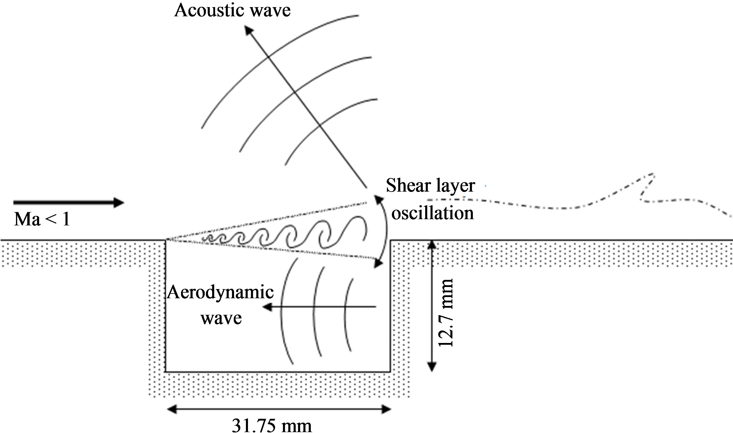
Figure 1. Schematic overview of the flow over the cavity.
approach. For detailed description of the used numerical techniques please look into the authors publications (e.g. [5].
2.1. CFD Code (LES-CFD)
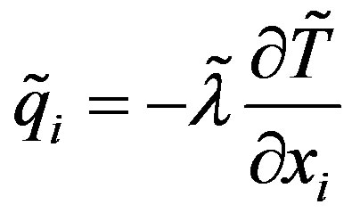
Although solving the U-RANS equations is possible for CAA computations (Dykas et al., 2008) the authors have decided to develop in-house CFD code into application of Large Eddy Simulation (LES) method. The LES equations for a compressible viscous flow are obtained by a decomposition of the variables of the Navier-Stokes equations into a Favre-filtered part ( , ˜) and an unresolved part (‘) that has to be modeled with a subgrid-scale (SGS) model. The Favre-filtered mass, momentum and energy equations can be written in the following differential form:
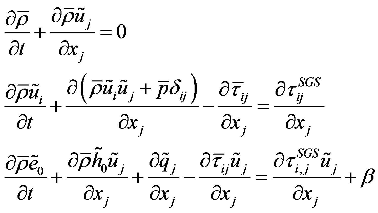 (1)
(1)
where β is the high-order, non-linear pressure-velocity subgrid term.
In the code, the Smagorinsky SGS-model was used, where
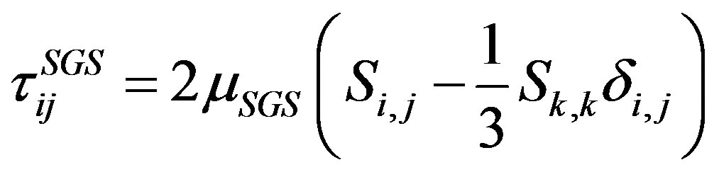
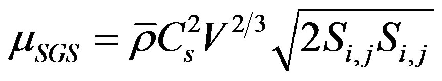
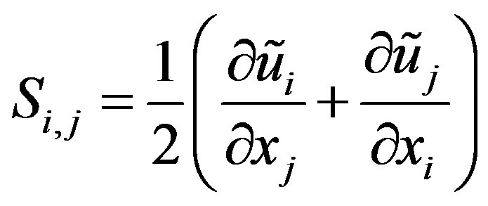
with μSGS the eddy viscosity, C = 0.18 the Smagorinsky constant and V is a volume of a grid cell.
2.2. Euler Acoustic Postprocessor (EAP-CAA)
For description of the aerodynamic noise generation and propagation in the mean flow, the full no-linear Euler equations have been chosen. These equations are formulated using decomposition of the actual variables into the mean flow parts (0) and fluctuating parts (‘). The conservative acoustic variables were in this case defined as:
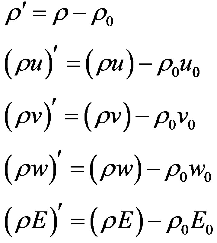 (2)
(2)
In the Cartesian coordinates, full Euler equations have a form:
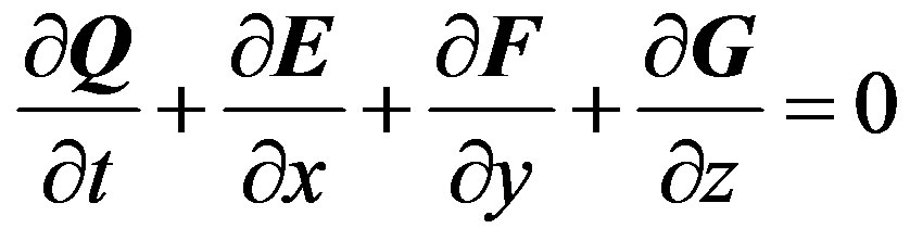 (3)
(3)
where vectors of conservative variables and fluxes can be written as follows:
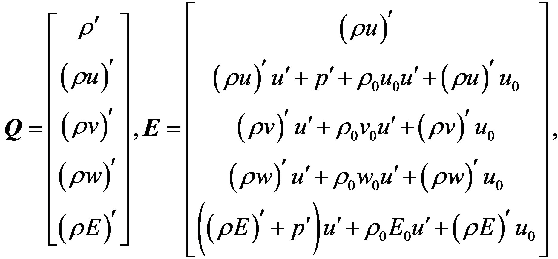
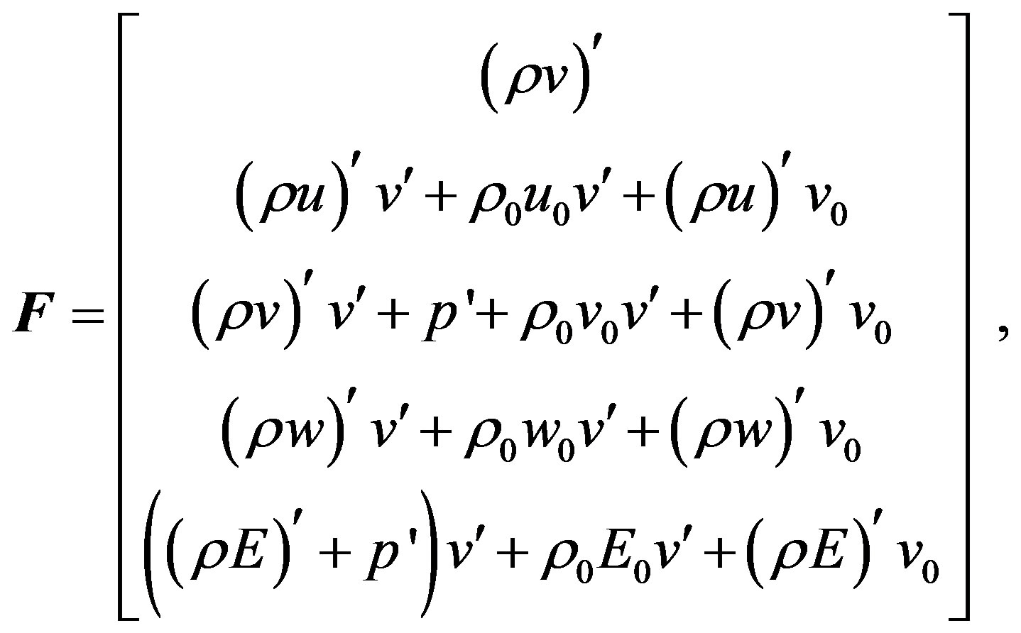
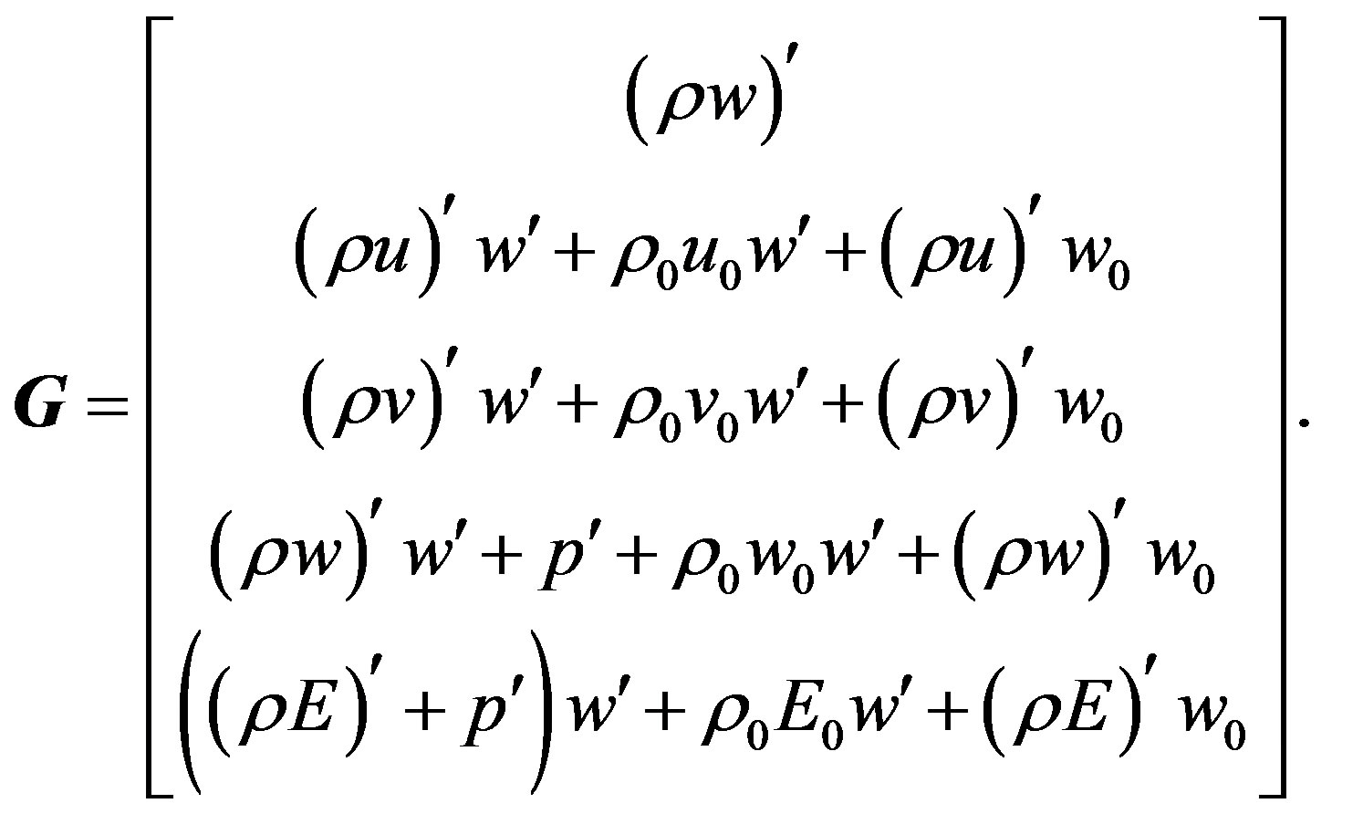
The relations for the primitive fluctuating variables in the function of the conservative fluctuating variables and mean values can be written in the form:
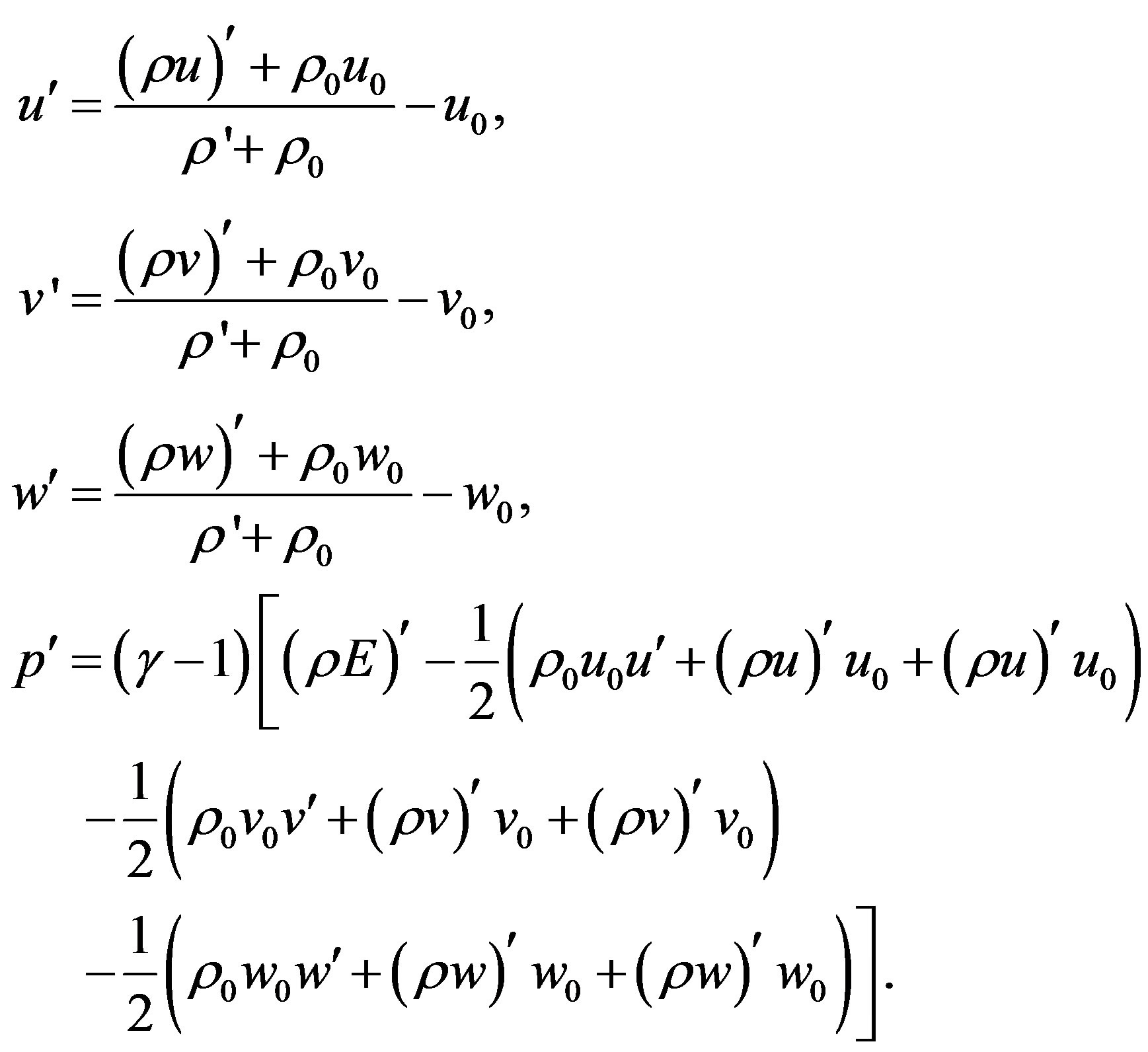 (4)
(4)
The presented Euler acoustic postprocessor is dedicated to the acoustic field assessment in the flows with wide range of Mach numbers, especially for the transonic internal flows.
3. Results of Computations
The cavity dimensions were assumed according to Ahuja and Medoza experiments (Ahuja and Medoza, 1964) (Figure 1). The length of the cavity is 31.75 mm and the depth is 12.7 mm. The ratio Lenght/Depth equal to 2.5 what makes possible to consider the acoustic field as 2D. Therefore in third direction, width of the cavity, only 10 control volumes was assumed. It allowed to decrease the computational time.
In the experiments, a jet flow over the cavity had a velocity of Ma = 0.53. For calculations the total parameters at the inlet were assumed as p0 = 121082.8926 Pa and T0 = 316.854 K, whereas the static pressure for outlet and exrapolating boundary conditions was 100,000 Pa.
3.1. LES Modeling
For LES modeling the in-house CFD code was used. The computational domain and boundary conditions used for modeling were presented in Figure 2. The structured numerical mesh comprising 7 blocks has ~1.2 M control volumes. For far-field boundaries the non-reflecting boundary conditions based on the extrapolating of the flow variables were applied.
The inlet is placed at 22.86 mm from the cavity leading edge and the height of the inlet is 12.7 mm.
The transient modeling was performed with a time step of 10–8 s. The unsteady flow field over the cavity was presented in the Figure 3" target="_self"> Figure 3 by means of Mach number contours. Both, the structure of the eddies of different scales inside the cavity and shear layer oscillation can be observed.
Figure 4 shows the acoustic pressure field obtained
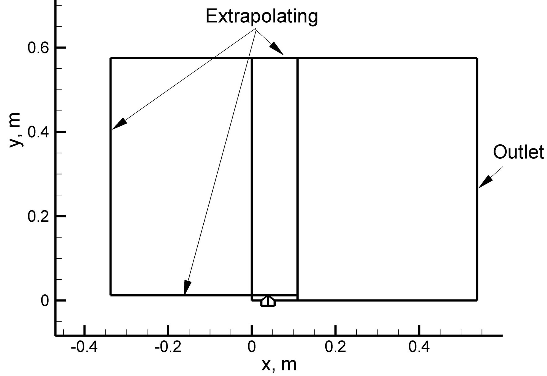

Figure 2. The computational domain of the cavity and boundary conditions for LES-CFD modeling.
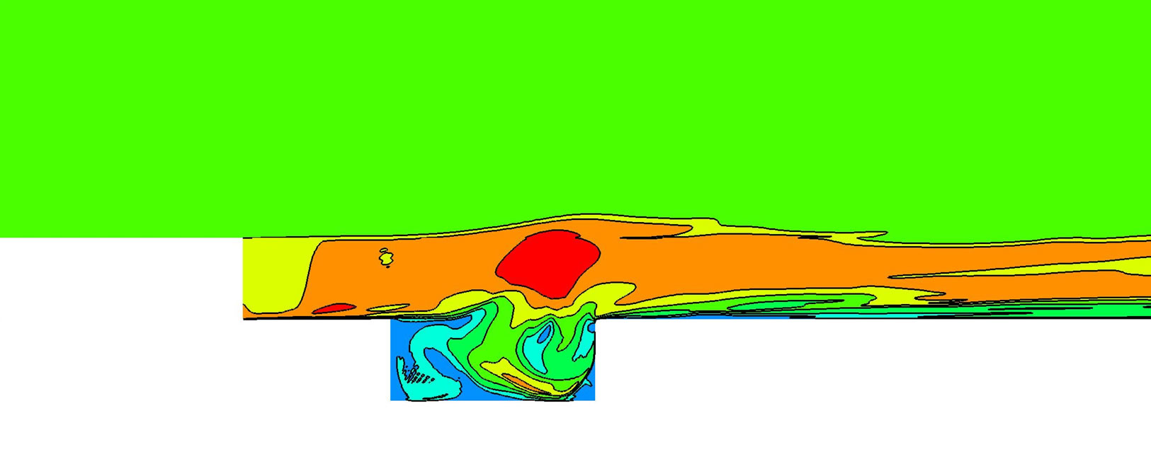
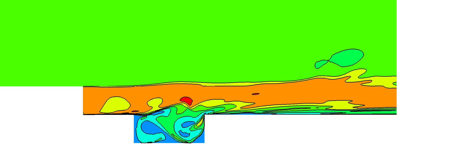
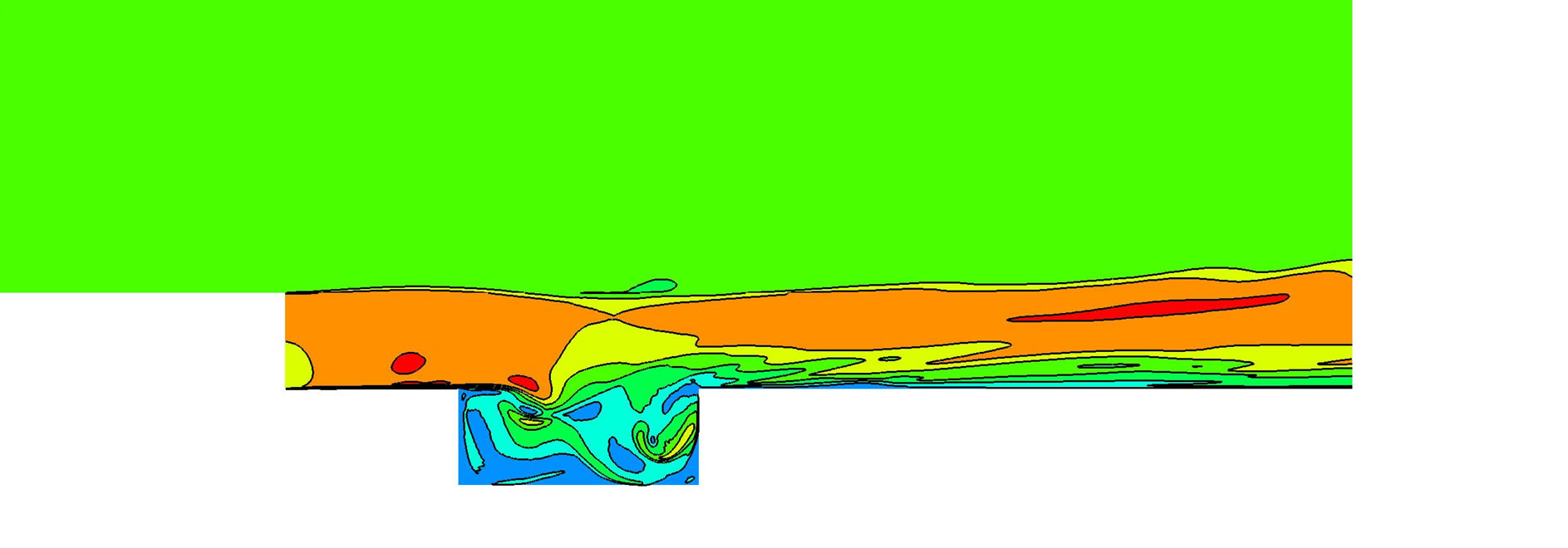
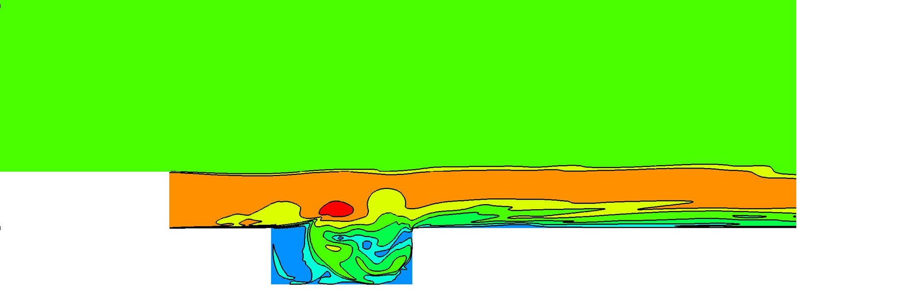
Figure 3.Snapshots of the Mach number field in and above cavity.
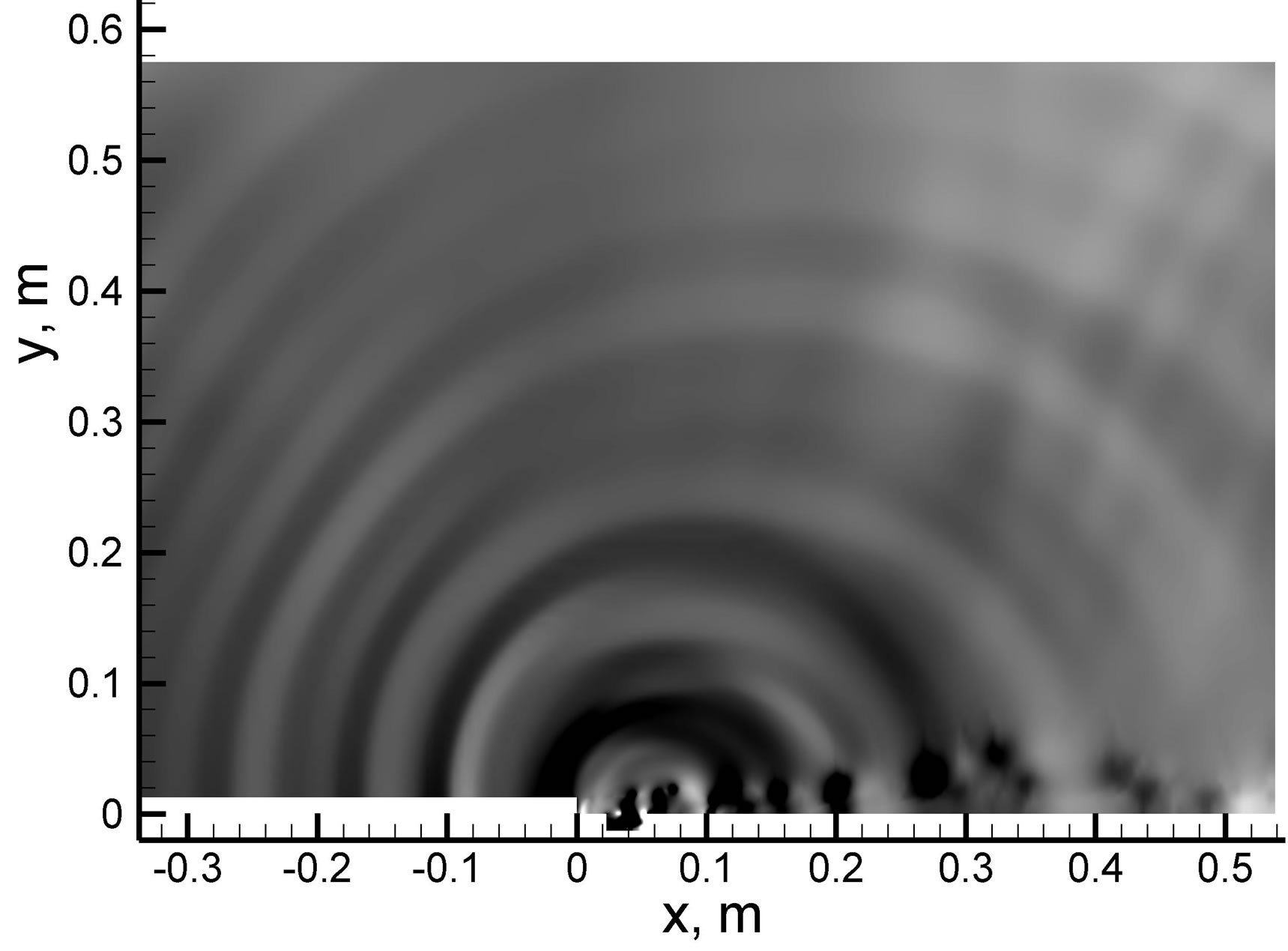
Figure 4. Snapshot of the acoustic pressure field from LES computations.
from LES calculations. Acoustic waves are mainly generated by the oscillation of the shear layer above cavity close to its trailing edge and propagated rather upstream.
3.2. Calculations Using Acoustic Postprocessor (EAP)
The computational domain and boundary conditions used for CAA modeling were presented in Figure 5. The structured numerical mesh includes 3 blocks with ~0.6 M control volumes. Two types of boundary conditions were used. For far-field boundaries the extrapolation of the flow variables were applied. From LES calculations the pressure variations have been used as boundary conditions for coupling of the CFD modeling with CAA calculations on the boundary.
For CAA analysis the transient CFD flow field from 10–3 s was taken into account and used as a CFD acoustic excitation boundary condition on a common surface. The CAA calculations were carried out with the same time step like in the case of LES modeling. The other method is based on an assumption of the instantaneous flow field from LES modeling (state “0” in Equation (2)), what is a better method in the case of aerodynamic noise modeling in a near field.
In the Figure 6 the acoustic pressure field obtained from CAA calculations was presented. The boundary condition for coupling of CFD results with CAA calculations was assumed very close to the cavity in order to check the ability of CAA in-house code for aerodynamic noise modeling in a near field. The picture of the acoustic field (Figure 6) shows differences in respect to the acoustic field obtained from LES modeling (Figure 4),
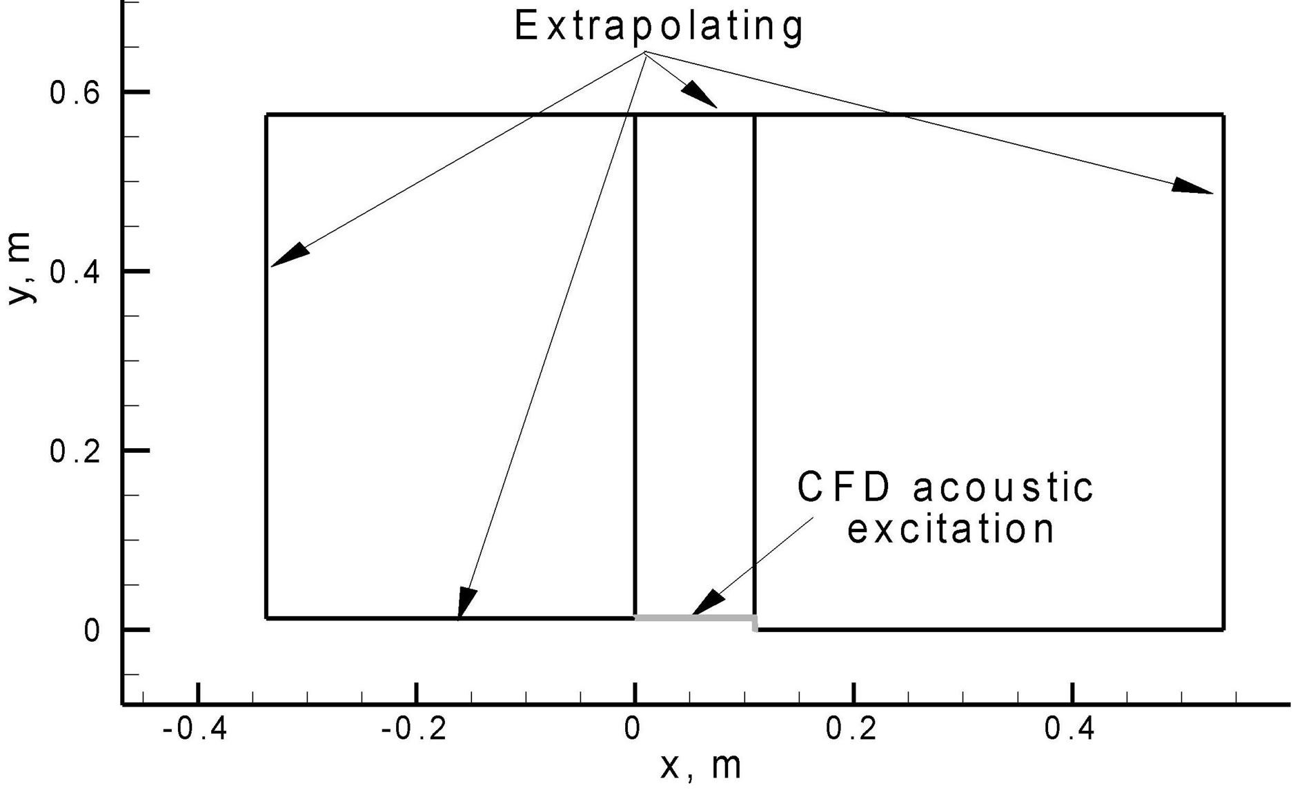
Figure 5. The computational domain of the cavity and boundary conditions for EAP-CAA modeling.
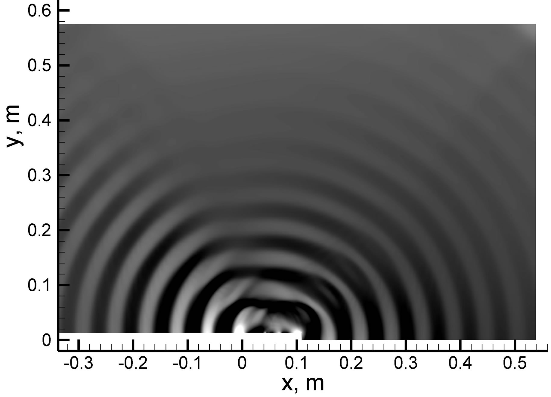
Figure 6. Snapshot of the acoustic pressure field from EAP computations.
what implies that the boundary conditions of CFD acoustic excitation should be assumed much further form the cavity. It means that for modeling the aerodynamic noise in a near field the boundary conditions for in-house acoustic postprocessor should be assumed not on the boundary only, but in whole computational domain (see Dykas et al., 2008). It allows to treat each point of the computational domain as a probable noise source.
3.3. FFT Analysis of the Results
The acoustic waves generated directly from LES computations and by means of CAA postprocessor have been analyzed in respect to the sound pressure level and their frequency. In the experiment of Ahuja and Mendoza (Ahuja and Mendoza, 1964) it was presented the SPL spectrum in a far field. Figure 7 shows the comparison of the SPL spectrum determined from LES and EAP results with experimental one in the point located at azimuthal angle 90˚. However, the distance of this point from the cavity in experiment was about 3.6 m, whereas in the case of presented calculations it was 0.36 m only. It had to affect the differences in value of Sound Pressure Level (SPL), what is visible in Figure 7. Moreover, the comparison of the SPL spectrum presented hereafter shows that by means of in-house codes it is possible to predict every other of main frequencies measured in experiment. This fact may be caused by the assumption of 2D character of the calculated phenomenon—limiting the size of the computational domain widthwise.
4. Conclusions
This paper deals with the numerical prediction of cavity
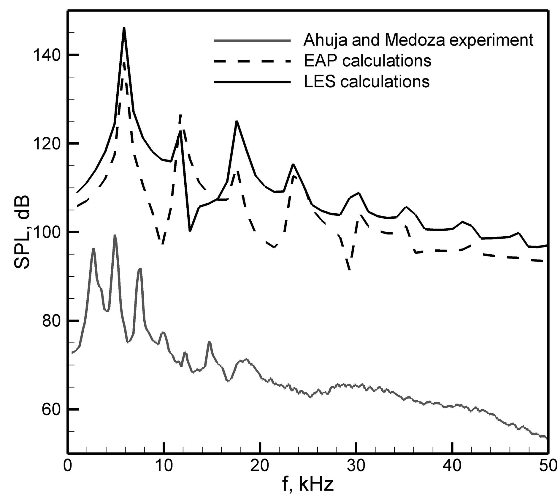
Figure 7. Comparison of the sound pressure level (SPL) far from the cavity.
flow noise using in-house CFD and CAA codes. The main target of the presented calculations was a qualitative estimation of the applied techniques in respect to the acoustic waves generation, their frequency and amplitude. The main attention was focused on the computational time assessment and determination of the boundary conditions for coupling between CFD and CAA computations. Both computations were carried out using the same size of the computational domain. The applied CAA technique is over 100 times less time consuming than LES method.
Presented in this paper results are the first step into the applications of the in-house CFD code basing on LES method for CAA calculations. Obtained first results show good qualitatively agreement between acoustic wave modeling using in-house CFD and CAA techniques. However, there is visible that in CAA calculations the position of boundary condition for CFD acoustic excitation was assumed too close to the cavity. For aerodynamic noise assessment in a near field the instantaneous flow variables from CFD calculations in whole computation domain should be used. The application of the extrapolating boundary conditions ensures the lack of the acoustic wave reflections.
Further investigations will concentrate on the quantitatively validation of the elaborated techniques (both LES and EAP). To this end the experimental results for cavity flows for various inlet Mach numbers will be used.
5. Acknowledgements
The authors would like to thank the Polish Ministry of Science and Higher Education for the financial support of the research project UMO-2011/01/B/ST8/03488.
REFERENCES
- S. Dykas, W. Wróblewski and T. Chmielniak, “Using a CFD/CAA Technique for Aerodynamic Noise Assessment,” Proceedings of ASME Turbo Expo 2008: Power for Land, Sea and Air GT2008, Berlin, 9-13 June 2008, pp. 784-794.
- S. Dykas, W. Wróblewski, S. Rulik and T. Chmielniak, “Numerical Modeling of the Acoustic Waves Propagation,” Archives of Acoustics, Vol. 35, No. 1, 2010, pp. 35- 48.
- K. K. Ahuja and J. Mendoza, “Effects of Cavity Dimensions, Boundary Layer, and Temperature on Cavity Noise with Emphasis on Benchmark Data to Validate Computational Aeroacoustic Codes,” 1964.
- S. Weyna, “An Acoustic Energy Dissipation of the Real Sources (in Polish),” 2005.
- W. Wróblewski, S. Dykas and A. Gepert, “Modeling of the Flows with Condensation (in Polish),” 2006.