ABSTRACT

In this article the computation of the Structured Singular Values (SSV) for the delay eigenvalue problems and polynomial eigenvalue problems is presented and investigated. The comparison of bounds of SSV with the well-known MATLAB routine mussv is investigated.

Keywords:

m-Values, Block Diagonal Uncertainties, Spectral Radius, Low-Rank Approximation, Delay Eigenvalue Problems, Polynomial Eigenvalue Problems

1. Introduction

The m-values [1] is an important mathematical tool in control theory; it allows discussing the problem arising in the stability analysis and synthesis of control systems to quantify the stability of a closed-loop linear time-invariant systems subject to structured perturbations. The structures addressed by the SSV is very general and allows covering all types of parametric uncertainties that can be incorporated into the control system by using real and complex Linear Fractional Transformations LFT’s. For more detail please see [1] - [7] and the references therein for the applications of SSV.

The versatility of the SSV comes at the expense of being notoriously hard, in fact Non-deterministic Polynomial time that is NP hard [8] to compute. The numerical algorithms which are being used in practice provide both upper and lower bounds of SSV. An upper bound of the SSV provides sufficient conditions to guarantee robust stability analysis of feedback systems, while a lower bound provides sufficient conditions for instability analysis of the feedback systems.

The widely used function mussv available in the Matlab Control Toolbox computes an upper bound of the SSV using diagonal balancing and Linear Matrix Inequality techniques [9] [10] . The lower bound is computed by using the generalization of power method developed in [11] [12] .

In this paper the comparison of numerical results to approximate the lower bounds of the SSV associated with mixed real and pure complex uncertainties is presented.

Overview of the article. Section 2 provides the basic framework. In particular, it explains how the computation of the SSV can be addressed by an inner-outer algorithm, where the outer algorithm determines the perturbation level and the inner algorithm determines a (local) extremizer of the structured spectral value set. In Section 3 it is explained that how the inner algorithm works for the case of pure complex structured perturbations. An important characterization of extremizers shows that one can restrict himself to a manifold of structured perturbations with normalized and low-rank blocks. A gradient system for finding extremizers on this manifold is established and analyzed. The outer algorithm is addressed in Section 4, where a fast Newton iteration for determining the correct perturbation level is developed. Finally, Section 5 presents a range of numerical experiments to compare the quality of the lower bounds to those obtained with mussv.

2. Framework

Consider a matrix where and an underlying perturba- tion set with prescribed block diagonal structure,

(1)

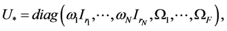
where denotes the identity matrix. Each of the scalars and the matrices may be constrained to stay real in the definition of. The integer N denotes the number of repeated scalar blocks (that is, scalar multiples of the identity) and F denotes the number of full blocks. This implies. In order to distinguish complex and real scalar blocks, assume that the first blocks are complex while the (possibly) remaining blocks are real. Similarly assume that the first full blocks are complex and the remaining blocks are real. The literature (see, e.g., [1] ) usually does not consider real full blocks, that is,. In fact, in control theory, full blocks arise from uncertainties associated to the frequency response of a system, which is complex-valued.

For simplicity, assume that all full blocks are square, although this is not necessary and our method extends to the non-square case in a straightforward way. Similarly, the chosen ordering of blocks should not be viewed as a limiting assumption; it merely simplifies notation.

The following definition is given in [1] , where denotes the matrix 2-norm and the identity matrix.

Definition 2.1. [13] . Let and consider a set. Then the SSV (or m-value) is defined as

(2)

In Definition 2.1, denotes the determinant of a matrix and in the following we make use of the convention that the minimum over an empty set is. In particular, if for all.

Note that is a positively homogeneous function, i.e.,

For, it follows directly from Definition 2.1 that.For general, the SSV can only become smaller and thus gives us the upper bound. This can be refined further by exploiting the properties of, see [14] . These relations between and, the largest singular value of A, justifies the name structured singular value for.

The important special case when only allows for complex perturb- ations, that is, and, deserves particular attention. In this case one can write instead of. Note that implies for any. In turn, there is such that if and only if there is, with the same norm, such that has the eigenvalue 1, which implies. This gives the following altern- ative expression:

(3)

where denotes the spectral radius of a matrix. For any nonzero eigenvalue of A, the matrix satisfies the constraints of the minimization problem shown in Equation (3). This establishes the lower bound

for the case of purely complex perturbations. Note that for. Hence, both the spectral radius and the

matrix 2-norm are included as special cases of the SSV.

2.1. A Reformulation Based on Structured Spectral Value Sets [13]

The structured spectral value set of with respect to a perturbation level is defined as

(4)

where denotes the spectrum of a matrix. Note that for purely complex, the set is simply a disk centered at 0. The set

(5)

allows us to express the SSV defined in Equation (2) as

(6)

that is, as a structured distance to singularity problem. This gives us that if and only if.

For a purely complex perturbation set, one can use Equation (3) to alternatively express the SSV as

(7)

where and one can have that, where deno- tes the open complex unit disk, if and only if.

2.2. Problem under Consideration [13]

Let us consider the minimization problem

(8)

where for some fixed. By the discussion above, the SSV, is the reciprocal of the smallest value of for which. This suggests a two-level algorithm: In the inner algorithm, we attempt to solve Equation (8). In the outer algorithm, we vary by an iterative procedure which exploits the knowledge of the exact derivative of an extremizer say with respect to. We address Equation (8) by solving a system of Ordinary Differential Equations (ODE’s). In general, this only yields a local minimum of Equation (8) which, in turn, gives an upper bound for and hence a lower bound for. Due to the lack of global optimality criteria for Equation (8), the only way to increase the robustness of the method is to compute several local optima.

The case of a purely complex perturbation set can be addressed ana- logously by letting the inner algorithm to determine a local optima for

(9)

where which then yields a lower bound for.

3. Pure Complex Perturbations [13]

In this section, we consider the solution of the inner problem discussed in

Equation (9) in the estimation of for and a purely complex

perturbation set

(10)

3.1. Extremizers

Now, make use of the following standard eigenvalue perturbation result, see, e.g., [15] . Here and in the following, denote.

Lemma 3.1. Consider a smooth matrix family and let be an eigenvalue of converging to a simple eigenvalue of as. Then is analytic near with

where and are right and left eigenvectors of associated to, that is, and.

Our goal is to solve the maximization problem discussed in Equation (9), which requires finding a perturbation such that is maximal among all with. In the following we call a largest eigenvalue if equals the spectral radius.

Definition 3.2. [13] . A matrix such that and has a largest eigenvalue that locally maximizes the modulus of is called a local extremizer.

The following result provides an important characterization of local extre- mizers.

Theorem 3.3. [13] . Let

be a local extremizer of. Assume that has a simple largest eigenvalue, with the right and left eigenvectors and scaled such that. Partitioning

(11)

such that the size of the components equals the size of the kth block in, additionally assume that

(12)

(13)

then

that is, all blocks of have unit 2-norm.

The following theorem allows us to replace full blocks in a local extremizer by rank-1 matrices.

Theorem 3.4. [13] . Let be a local ext- remizer and let be defined and partitioned as in Theorem 3.3. Assuming that Equation (13) holds, every block has a singular value 1 with associated

singular vectors and for some

. Moreover, the matrix

is also a local extremizer, i.e.,.

Remark 3.1. [13] . Theorem 3.3 allows us to restrict the perturbations in the structured spectral value set shown in Equation (4) to those with rank-1 blocks, which was also shown in [1] . Since the Frobenius and the matrix 2-norms of a rank-1 matrix are equal, one can equivalently search for extremizers within the submanifold

(14)

3.2. A system of ODEs to Compute Extremal Points of [13]

In order to compute a local maximizer for, with, First construct a matrix valued function such that a largest eigenvalue of has maximal local increase. Then derive a system of ODEs satisfied by this choice of.

Orthogonal projection onto. In the following, we make use of the Frobenius inner product for two matrices. Let

(15)

denote the orthogonal projection, with respect to the Frobenius inner product, of a matrix onto. To derive a compact formula for this projection, use the pattern matrix

(16)

where denotes the -matrix of all ones.

Lemma 3.5. [13] . For, let

denote the block diagonal matrix obtained by entrywise multiplication of C with

the matrix defined in Equation (20). Then the orthogonal projection of C

onto is given by

(17)

where, and.

The local optimization problem [13] . Let us recall the setting from Section (3.1): assume that is a simple eigenvalue with eigenvectors normalized such that

(18)

As a consequence of Lemma 3.1, see also Equation (15), to have

(19)

where and the dependence on t is intentionally omitted.

Letting, with as in Equation (18), now we aim at determ- ining a direction that locally maximizes the increase of the modulus of. This amounts to determining

(20)

as a solution of the optimization problem

(21)

The target function in Equation (20) follows from Equation (19), while the constraints in Equation (21) ensure that is in the tangent space of at. In particular Equation (20) implies that the the norms of the blocks of are conserved. Note that Equation (20) only becomes well-posed after imposing an additional normalization on the norm of U. The scaling chosen in the following lemma aims at.

Lemma 3.6. [13] . With the notation introduced above and partitioned as in Equation (11), a solution of the optimization problem discussed in Equa- tion (20) is given by

(22)

with

(23)

(24)

Here, is the reciprocal of the absolute value of the right-hand side in Equation (23), if this is different from zero, and otherwise. Similarly, is the reciprocal of the Frobenius norm of the matrix on the right hand side in Equation (24), if this is different from zero, and otherwise. If all right-hand sides are different from zero then.

Corollary 3.7. [13] . The result of Lemma 3.6 can be expressed as

(25)

where is the orthogonal projection and are diagonal

matrices with positive.

Proof. The statement is an immediate consequence of Lemma 3.5.

The system of ODEs. Lemma 3.6 and Corollary 3.7 suggest to consider the following differential equation on the manifold:

(26)

where is an eigenvector, of unit norm, associated to a simple eigenvalue of for some fixed. Note that depend on as well. The differential Equation (30) is a gradient system because, by definition, the right-hand side is the projected gradient of.

The following result follows directly from Lemmas 3.1 and 3.6.

Theorem 3.8. [13] . Let satisfy the differential Equation (26). If is a simple eigenvalue of, then increases monotonically.

The following lemma establishes a useful property for the analysis of stationary points of Equation (26).

Lemma 3.9. [13] . Let satisfy the differential Equation (26). If is a nonzero simple eigenvalue of, with right and left eigen- vectors and scaled, then

(27)

where.

Remark 3.3. The choice of, originating from Lemma 3.6., to achieve unit norm of all blocks in Equation (25), is completely arbitrary. Other choices would be also acceptable and investigating an optimal one in terms of speed of convergence to stationary points would be an interesting issue.

The following result characterizes stationary points of Equation (26).

Theorem 3.10. [13] . Assume that is a solution of Equation (26) and is a largest simple nonzero eigenvalue of with right/left eigen- vectors,. Moreover, suppose that Assumptions (12) and (13) hold for and. Then

(28)

for a specific real diagonal matrix. Moreover if has (locally) maximal modulus over the set then D is positive.

3.3. Projection of Full Blocks on Rank-1 Manifolds [13]

In order to exploit the rank-1 property of extremizers established in Theorem 3.4, one can proceed in complete analogy to [16] in order to obtain for each full block an ODE on the manifold M of (complex) rank-1 matrices. The derivation of this system of ODEs is straightforward; the interested reader can see [17] for full details.

The monotonicity and the characterization of stationary points follows analogously to those obtained for Equation (26); and also refer to [16] for the proofs. As a consequence one can use the ODE in Equation (28) instead of Equation (26) and gain in terms of computational complexity.

3.4. Choice of Initial Value Matrix and [13]

In our two-level algorithm for determining use the perturbation obtained for the previous value as the initial value matrix for the system of ODEs. However, it remains to discuss a suitable choice of the initial values and in the very beginning of the algorithm.

For the moment, let us assume that A is invertible and write

which aim to have as close as possible to singularity. To determine, one can perform an asymptotic analysis around. For this purpose, let us consider the matrix valued function

and let denote denote an eigenvalue of with smallest modulus. Letting v and w denote the right and left eigenvectors corresponding to, scaled such that, Lemma 3.1 implies

In order to have the locally maximal decrease of at choose

(29)

where the positive diagonal matrix D is chosen such that. This is always possible under the genericity assumptions (12) and (13). The orthogonal projector onto can be expressed in analogy to Equation (21) for

, with the notable difference that for.

Note that there is no need to form; v and w can be obtained as the eigenvectors associated to a largest eigenvalue of A. However, attention needs to

be paid to the scaling. Since the largest eigenvalue of A is, w and v have

to be scaled accordingly.

A possible choice for is obtained by solving the following simple linear equation, resulting from the first order expansion of the eigenvalue at:

This gives

(30)

This can be improved in a simple way by computing this expression for for several eigenvalues of A (say, the m largest ones) and taking the smallest computed. For a sparse matrix A, the matlab function eigs (an interface for ARPACK, which implements the implicitly restarted Arnoldi Method [18] [19] allows to efficiently compute a predefined number m of Ritz values.

Another possible, very natural choice for is given by

(31)

where is the upper bound for the SSV computed by the matlab function mussv.

4. Fast Approximation of [13]

This section discuss the outer algorithm for computing a lower bound of. Since the principles are the same, one can treat the case of purely complex perturbations in detail and provide a briefer discussion on the extension to the case of mixed complex/real perturbations.

Purely Complex Perturbations

In the following let denote a continuous branch of (local) maximizers for

computed by determining the stationary points of the system of ODEs in Equation (30). The computation of the SSV is equivalent to the smallest solution of the equation. In order to approximate this solution, aim at computing such that the boundary of the -spectral value set is locally

contained in the unit disk and its boundary is tangential to the unit

circle. This provides a lower bound for.

Now make the following generic assumption.

Assumption 4.1. [13] . For a local extremizer of, with corresponding largest eigenvalue, assume that is simple and that and are smooth in a neighborhood of.

The following theorem gives an explicit and easily computable expression for the derivative of.

Theorem 4.1. [13] . Suppose that Assumption 4.1 holds for and. Let and be the corresponding right and left eigen- vectors of, scaled according to Equation (22). Consider the partitioning of, , and suppose that Assumptions (12) and (13) hold. Then

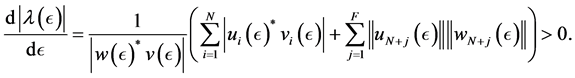(32)

5. Numerical Experimentation

This section provides the comparison of the lower bounds of SSV computed by well-known Matlab function mussv and the algorithm [13] .

We consider the following delay eigenvalue problem of the form:

where,

and.

Example 1. Consider the following two dimensional matrix taken from above mentioned delay eigenvalue problem.

along with the perturbation set

Apply the Matlab routine mussv, one can obtain the perturbation with

and For this example, one can obtain the upper bound while the same lower bound as.

By using the algorithm [13] , one can obtain the perturbation with

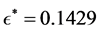and while. The same lower bound can be obtained as the one obtained by mussv.

In the following Table 1, it is presented the comparison of the bounds of SSV computed by MUSSV and the algorithm [13] for the matrix given bellow. In the very first column, it is presented the dimension of the matrix. In the second column, it is presented the set of block diagonal matrices denoted by BLK. In the third, fourth and fifth columns, it is presented the upper and lower bounds, computed by MUSSV and the lower bound computed by algorithm [13] respectively.

and

Example 2. Consider the following two dimensional matrix taken from above mentioned delay eigenvalue problem.

along with the perturbation set

Apply the Matlab routine mussv, one can obtain the perturbation with

and For this example, one can obtain the upper bound while the same lower bound as.

By using the algorithm [13] , one can obtain the perturbation with

and while The same lower bound can be obtained as the one obtained by mussv.

In Table 2, it is presented the comparison of the bounds of SSV computed by MUSSV and the algorithm [13] for the matrix given bellow. In the very first column, it is presented the dimension of the matrix. In the second column, it is presented the set of block diagonal matrices denoted by BLK. In the third, fourth and fifth columns, it is presented the upper and lower bounds, computed by MUSSV and the lower bound computed by algorithm [13] respectively.

and

We consider the polynomial eigenvalue problems.

Consider the quadratic eigenvalue problem of the form:

Example 3. Consider the following three dimensional matrix taken from above mentioned delay eigenvalue problem.

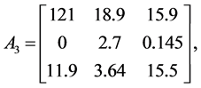
along with the perturbation set

Apply the Matlab routine mussv, one can obtain the perturbation with

and For this example, one can obtain the upper bound while the same lower bound as

By using the algorithm [13] , one can obtain the perturbation with

and while The same lower bound can be obtained as the one obtained by mussv.

In Table 3, it is presented the comparison of the bounds of SSV computed by MUSSV and the algorithm [13] for the matrix given bellow. In the very first column, it is presented the dimension of the matrix. In the second column, it is presented the set of block diagonal matrices denoted by BLK. In the third, fourth and fifth columns, it is presented the upper and lower bounds, computed by MUSSV and the lower bound computed by algorithm [13] respectively.

and

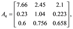
Example 4. Consider the following three dimensional matrix taken from above mentioned delay eigenvalue problem.

along with the perturbation set

Apply the Matlab routine mussv, one can obtain the perturbation with

and For this example, one can obtain the upper bound while the same lower bound as

By using the algorithm [13] , one can obtain the perturbation with

and while The same lower bound can be obtained as the one obtained by mussv.

In Table 4, it is presented the comparison of the bounds of SSV computed by MUSSV and the algorithm [13] for the matrix given bellow. In the very first column, it is presented the dimension of the matrix. In the second column, it is presented the set of block diagonal matrices denoted by BLK. In the third, fourth and fifth columns, it is presented the upper and lower bounds, computed by MUSSV and the lower bound computed by algorithm [13] respectively.

and

Example 5. Consider the following three dimensional matrix taken from above mentioned delay eigenvalue problem.

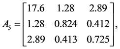
along with the perturbation set

Apply the Matlab routine mussv, one can obtain the perturbation with

and For this example, one can obtain the upper bound while the same lower bound as.

By using the algorithm [13] , one can obtain the perturbation with

and while The same lower bound can be obtained as the one obtained by mussv.

In Table 5, it is presented the comparison of the bounds of SSV computed by MUSSV and the algorithm [13] for the matrix given bellow. In the very first column, it is presented the dimension of the matrix. In the second column, it is presented the set of block diagonal matrices denoted by BLK. In the third, fourth and fifth columns, it is presented the upper and lower bounds, computed by MUSSV and the lower bound computed by algorithm [13] respectively.

and

6. Conclusion

In this article the problem of approximating structured singular values for the delay eigenvalue and polynomial eigenvalue problems is considered. The obtained results provide a characterization of extremizers and gradient systems, which can be integrated numerically in order to provide approximations from below to the structured singular value of a matrix subject to general pure complex and mixed real and complex block perturbations. The experimental results show the comparison of the lower bounds of structured singular values with once computed by MUSSV and alogorithm [13] .

Cite this paper

Rehman, M.-U., Majeed, D., Nasreen, N. and Tabassum, S. (2017) Computing Structured Singular Values for Delay and Polynomial Eigenvalue Problems. Open Journal of Applied Sciences, 7, 348-364. https://doi.org/10.4236/ojapps.2017.77028

References

- 1. Packard, A. and Doyle, J. (1993) The Complex Structured Singular Value. Automatica, 29, 71-109.
https://doi.org/10.1016/0005-1098(93)90175-S - 2. Bernhardsson, B. and Rantzer, A. and Qiu, L. (1994) Real Perturbation Values and Real Quadratic Forms in a Complex Vector Space. Linear Algebra and Its Applications, 1, 131-154.
- 3. Chen, J., Fan, M.K.H. and Nett, C.N. (1996) Structured Singular Values with Nondiagonal Structures. I. Characterizations. IEEE Transactions on Automatic Control, 41, 1507-1511.
- 4. Hinrichsen, D. and Pritchard, A.J. (2005) Mathematical Systems Theory I, Vol. 48 of Texts in Applied Mathematics. Springer-Verlag, Berlin.
- 5. Karow, M., Kokiopoulou, E. and Kressner, D. (2010) On the Computation of Structured Singular Values and Pseudospectra. Systems & Control Letters, 59, 122-129.
https://doi.org/10.1016/j.sysconle.2009.12.007 - 6. Karow, M., Kressner, D. and Tisseur, F. (2006) Structured Eigenvalue Condition Numbers. SIAM Journal on Matrix Analysis and Applications, 28, 1052-1068.
https://doi.org/10.1137/050628519 - 7. Qiu, L., Bernhardsson, B., Rantzer, A., Davison, E.J., Young, P.M. and Doyle, J.C. (1995) A Formula for Computation of the Real Stability Radius. Automatica, 31, 879-890.
- 8. Braatz, R.P., Young, P.M., Doyle, J.C. and Morari, M. (1994) Computational Complexity of µ Calculation. IEEE Transactions on Automatic Control, 39, 1000-1002.
- 9. Fan, M.K.H., Tits, A.L. and Doyle, J.C. (1991) Robustness in the Presence of Mixed Parametric Uncertainty and Unmodeled Dynamics. IEEE Transactions on Automatic Control, 36, 25-38.
- 10. Young, P.M., Newlin, M.P. and Doyle, J.C. (1992) Practical Computation of the Mixed µ Problem. American Control Conference, 24-26 June 1992, 2190- 2194.
- 11. Packard, A., Fan, M.K.H. and Doyle, J. (1998) A Power Method for the Structured Singular Value. Proceedings of the 27th IEEE Conference on Decision and Control, 7-9 December 1988, 2132-2137.
- 12. Young, P.M., Doyle, J.C., Packard, A., et al. (1994) Theoretical and Computational Aspects of the Structured Singular Value. Systems, Control and Information, 38, 129-138.
- 13. Guglielmi, N., Rehman, M.-U. and Kressner, D. (2016) A Novel Iterative Method to Approximate Structured Singular Values. arXiv preprint arXiv:1605.04103.
- 14. Zhou, K., Doyle, J. and Glover, K. (1996) Robust and Optimal Control. Prentice Hall, New Jersey, Volume 40.
- 15. Kato, T. (2013) Perturbation Theory for Linear Operators. Springer Science & Business Media, Volume 132.
- 16. Guglielmi, N. and Lubich, C. (2011) Differential Equations for Roaming Pseudospectra: Paths to Extremal Points and Boundary Tracking. SIAM Journal on Numerical Analysis, 49, 1194-1209.
https://doi.org/10.1137/100817851 - 17. Guglielmi, N, and Lubich, C. (2013) Low-Rank Dynamics for Computing Extremal Points of Real Pseudospectra. SIAM Journal on Matrix Analysis and Applications, 34, 40-66.
https://doi.org/10.1137/120862399 - 18. Lehoucq, R.B. and Sorensen, D.C. (1996) Deflation Techniques for an Implicitly Restarted Arnoldi Iteration. SIAM Journal on Matrix Analysis and Applications, 17, 789-821.
https://doi.org/10.1137/S0895479895281484 - 19. Lehoucq, R.B., Sorensen, D.C. and Yang, C. (1998) ARPACK Users’ Guide: Solution of Large-Scale Eigenvalue Problems with Implicitly Restarted Arnoldi Methods. SIAM, Volume 6.