Open Journal of Applied Sciences
Vol.05 No.04(2015), Article ID:55880,9 pages
10.4236/ojapps.2015.54014
Numerical Solution of Second-Order Linear Fredholm Integro-Differetial Equations by Trigonometric Scaling Functions
Hamid Safdari, Yones Esmaeelzade Aghdam
Department of Mathematics, Shahid Rajaee Teacher Training University, Tehran, Iran
Email: HSafdari@srttu.edu, yonesesmaeelzade@gmail.com
Copyright © 2015 by authors and Scientific Research Publishing Inc.
This work is licensed under the Creative Commons Attribution International License (CC BY).
http://creativecommons.org/licenses/by/4.0/


Received 17 March 2015; accepted 13 April 2015; published 22 April 2015
ABSTRACT
The main aim of this paper is to apply the Hermite trigonometric scaling function on [0, 2p] which is constructed for Hermite interpolation for the linear Fredholm integro-differential equation of second order. This equation is usually difficult to solve analytically. Our approach consists of reducing the problem to a set of algebraic linear equations by expanding the approximate solution. Some numerical example is included to demonstrate the validity and applicability of the presented technique, the method produces very accurate results, and a comparison is made with exiting re- sults. An estimation of error bound for this method is presented.
Keywords:
Numerical Technique, Fredholm Integro-Differential Equations, Hermite Trigonometric Wavelets, Operational Matrix, Error Estimates

1. Introduction
In this paper we solve the Fredholm Linear Integro-Differential Equations as
 (1)
(1)
where ,
,  , and
, and  are given functions that have suitable derivatives, and
  and
and  are given real constans. In most situations, it is difficult to obtain exact solution of the above integration. Hence various approximation method have been proposed and studied. The purpose of the present paper is to develop a trigonometric Hermite wavelet approximation for the computing of the problem [1] .
Systems of integro-differential equations have a major role in the fields of science, physical phenomena, and engineering, such as nano-hydrodynamics, glass-forming process, dropwise condensation, wind ripple in the de- sert, and modeling the competition between tumor cells and the immune system. The concept of a system of integro-differential equations has motivated a huge amount of research work in recent years. Alot of attention has been devoted to the study of differential-difference equations, e.g. equations containing shifts of the un- known function and its derivates, and also integro-differential-difference equations. For instance, see [2] [3] . There are several numerical methods for solving system of linear integro-differential equations, for example, the rationalized Haar functions method [4] , Galerkin methods with hybrid functions [5] , the spline approximation method [6] , the Chebyshev polynomial method [7] , the spectral method [8] , the CAS wavelet method [9] , Ruge- Kutta methods [10] , the Adomian decomposition methods [11] , and the interested reader can see [12] [13] for more published research works in the subject.
Our approach consists of reducing the problem to a set of linear equations by trigonometric scaling functions which is constructed for Hermite interpolation. A difficulty of using wavelet for the representation of integral operators is that quadrature leads to potentially high cost with sparse matrix. This fact particularly encourages us in efforts to devote to some appropriate wavelet bases to simplify the computation expense of the reoresentation matrix, which is importent to improve the wavelet method. Recently, the trigonometric interpolant wavelet has arisen in the approximation of operators [14] - [16] . Quack [17] has constructed a multiresolution analysis (MRA). Chen [18] [19] presented the feasibility of trigonometric wavelet numerical methods for stokes problem and Hadamard integral equation.
The organization of the rest of this paper is as follows: Section (0) describe the trigonometric scaling function on , and construct the operational matrix of derivative for these function. Section (0) summarizes the application of trigonometric scaling functions to the solution of Problem (1). Thus, a set of linear equations is formed and a solution of the considered problem is introduced. In Section (0), we report our computational results and demonstrate the accuracy of the proposed numerical schemes by presenting numerical examples. Note that we have computed the numerical results by MATLAB programming.
2. Interpolatory Hermite Trigonometric Wavelets
In this section, we will give a brief introduction of Quak’s work on the construction of Hermite interpolatory trigonometric wavelets and their basic properties. More details can be found in (see [17] ).
For all , two scaling functions
  and
and  are defined as
 (2)
(2)
 (3)
(3)
where the Dirichlet kernel  and its conjugate kernel
  are defined as

Obviously,  , where
  is the linear space of trigonometric polynomials with degree not
exceeding l. The equally spaced nodes on the interval  with a dyadic step are denoted by
 , for
, for
any  and
and , where
  is the set of all non-negative integers. Let
 , for
, for , and
, and .
.
Lemma 1 (See [17] .) For  we have


and their derivations are given by


Theorem 1 (Interpolatory properties of the scaling functions). (See [17] ) For , the following inter- polatory properties hold for each
 (4)
(4)
From above we can take wavelet functions  as scaling functions. Now, we can define the scaling function spaces
 . Then we have
Definition 2 (Scaling functions space). For all  define the wave space
  as follows

As a first step of studying the spaces , the following result identifies the trigonometric polynomials which from alternative bases of these spaces.
Now a Hermite-type project operator can be introduced by means of the scaling functions. For all  the Hermite projection operators
  mapping any real-valued differentiable
  -periodic function f into the space
  is defined as
 (5)
(5)
where ,
,  , C, and
  are vectors with dimension
 . The following properties of the operators
  are therefore obvious:


Theorem 3 Let , and its trigonometric wavelet approximation is
 , then we have

where C is a positive constant value.
Proof. See [17] .
Lemma 2 (The operational matrix of scaling function derivative). (See [20] ) The differentiation of vector  in 5 can be expressed as [20]

where  is
is  operational matrix of derivative for trigonometric scaling function. Suppose
 (6)
(6)
where  and
and . So the matrix
  can be respresented as a block matrix as

where  and
and  are
are  matrices. The entries of matrices
  and
and  may be find by using

where  is a
is a  zero matrix,
  is a
is a  identity matrix. Using
  we get
 (7)
(7)
Using 7 and  we get
 (8)
(8)
and
 (9)
(9)
for .
.
3. Procedure Solution Using the Trigonometric Scaling Function
In this section, we first give the computational schemes for Equation (1) with the Newton-Cotes formulas. For either one of these rules, we can make a more accurate approximation by breaking up the interval  into some number N of subintervals. This is called a composite rule, extended rule, or iterated rule. For example, the composite trapezoidal rule for the discretization form of (1) can be stated as
 (10)
(10)
where the subintervals have the form , with
  and
and . By introducing a
basis  for the subspace
 , the coefficients vector
  of the discrete solution is defined by
 (11)
(11)
where C is  unknown vector defined similar to (5). By substituting
  and using Lemma (2) in (1) we have a linear system. Now for determining unknown coefficients vector C or
  and
and , we choose collo- cation method with choosing collocation points as
 (12)
(12)
Thus we have
 (13)
(13)
By using Lemma 2 and after summarizing Equation (13) can be rewritten as the matrix form  where
where ,
,  , and
, and . Now, let us calculate the entries
  and
and  in the system matrix.


where the matrix ,
,  ,
,  , and
, and  defined in Lemma (2), and I is a
  identity matrix. So the unknown function
  can be found. Note that we find these function by MATLAB.
4. Numerical Example
To support our theoretical discussion, we applied the method presented in this paper to several examples. The main objective here is to solve these two examples using the trigonometric scaling function and compare our results with exact solution.
Example 4 Consider the second-order the Fredholm Linear Integro-Differential Equation

with the mixed conditions  and
and . The exact solution of this problem is
 . We
. We
apply the suggested method with  and
and . The behavior of the approximate solution using the proposed method with
 ,
,  and the exact solution are presented in Figure 1. In Table 1, we give the errors
  of matrix A for different values of J. From this figure, it is clear that the proposed method can be considered as an efficient method to solve the linear integral equations. From Table 1 we see the errors decrease rapidly as J increase.
In Table 2 we compare the new method with ,
,  and
and  together with the exact solution. For the purpose of comparison we defined the meximum error for
  as
as

Example 5 Consider the following second-order the Fredholm Linear Integro-Differential Equation

with the initial conditions ,
,  and exact solution
 . This problem is solved by the same me- thods applied in example (4). Results are shown in Figure 2. From this figure, it is clear that the proposed method can be considered as an efficient method to solve the linear integral equations. For the purpose of com- parison in Table 3 we give the errors
  of matrix A for different values of J. From Table 4 we see the errors decrease rapidly as J increase. In Table 4 we compare the new method with J = 1, J = 2 and J = 3 together with the exact solution.

Table 1. The maximum error matrix A from Example 4.
Table 2. Error analysis and numerical results of Example 4.
Table 3. The maximum error matrix A from Example 5.
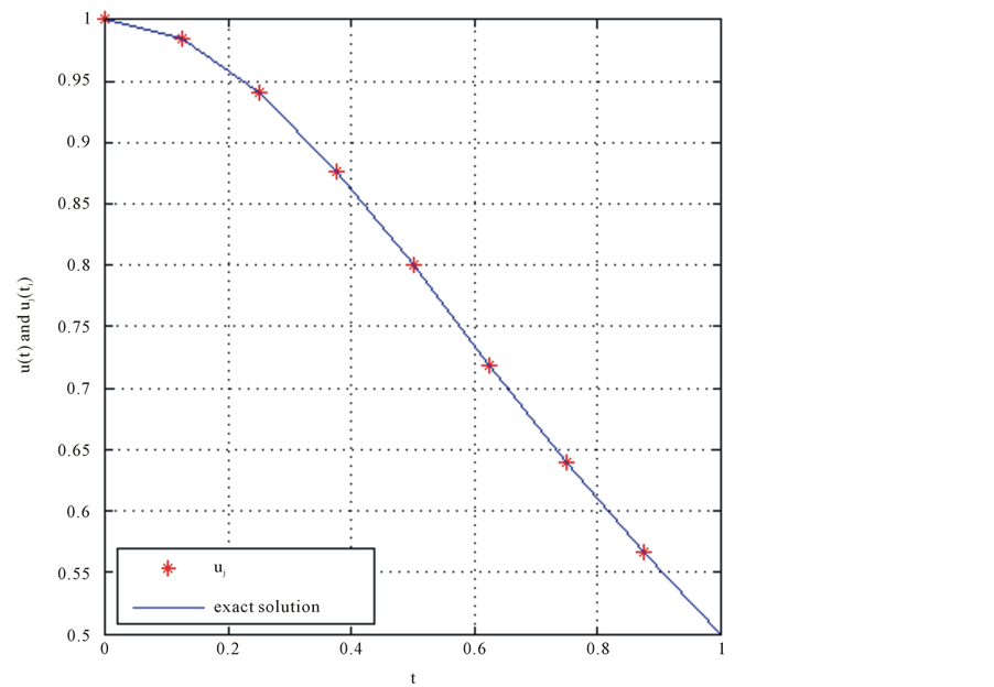
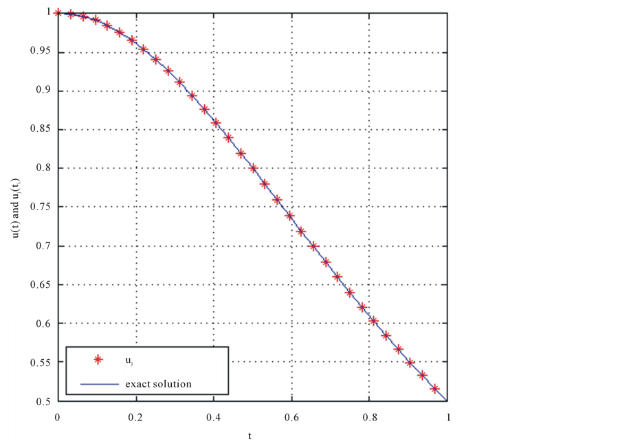
Figure 1. Result EX.4 for J = 1 and N = 7; Result EX.4 for J = 2 and N = 7.
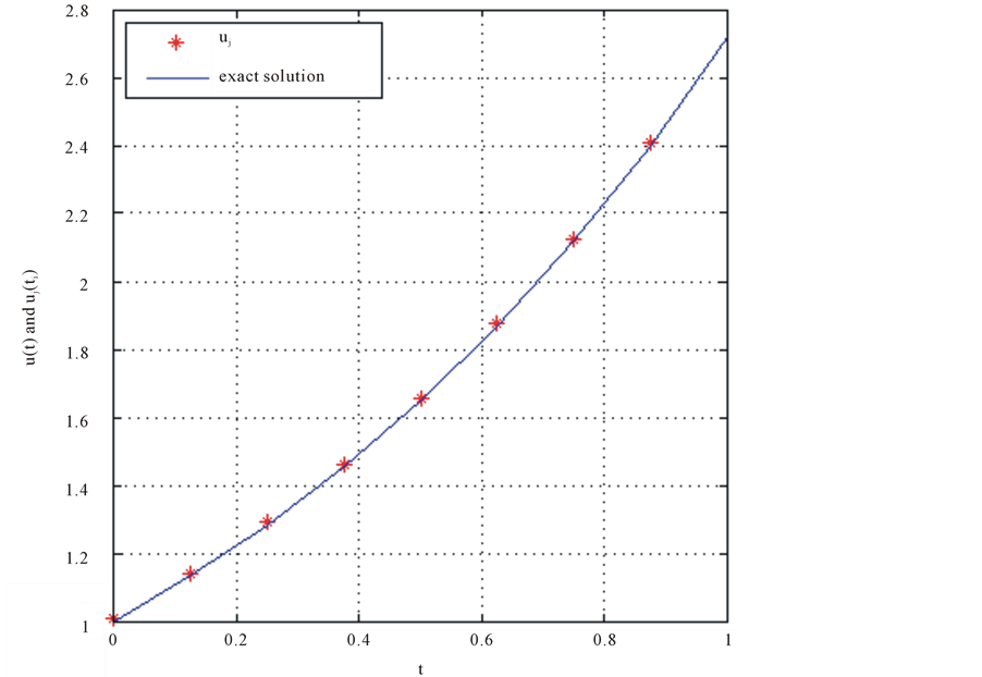
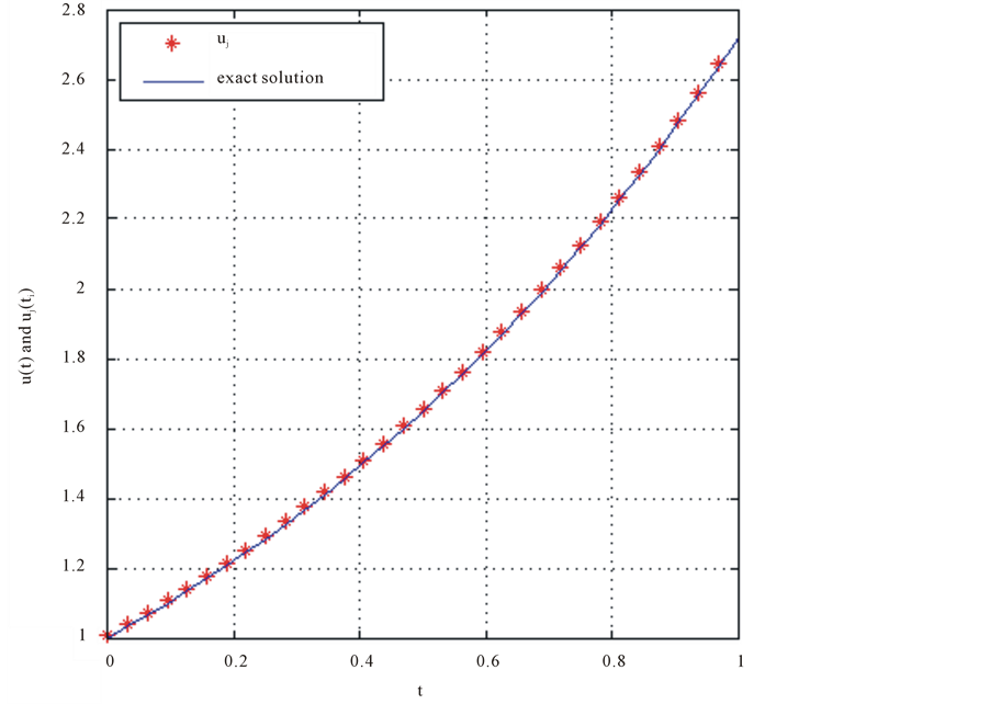
Figure 2. Result EX.5 for J = 1 and N = 7; Result EX.5 for J = 2 and N = 7.
Table 4. Error analysis and numerical results of Example 5.
5. Conclusion
Our results indicate that the method with the trigonometric scaling bases can be regarded as a structurally simple algorithm that is conventionally applicable to the numerical solution of IDEs. In addition, although we have re- stricted our attention to linear Fredholm IDEs, we expect the method to be easily extended to more general IDEs. the presented method which is based on the trigonometric scaling function is proposed to find the approximate solution. A comparison of the exact solution reveals that the presented method is very effective and convenient. Nevertheless, as Figure 1 and Figure 2 illustrate, the error of the trigonometric scaling bases shows that the accuracy improves with increasing J, hence for better results, using number J is recommended. Also form the obtained approximate solution, we can conclude that the proposed method gives the solution in an excellent agree- ment with the exact solution. All computations are done using MATLAB programming.
Acknowledgements
The authors are very grateful to the editor for carefully reading the paper and for their comments and sugges- tions which have improved the paper.
References
- Desmond, R.A., Weiss, H.L., Arani, R.B., Soong, S.-J., Wood, M.J., Fiddian, P., Gnann, J. and Whitley, R.J. (2002) Clinical Applications for Change-Point Analysis of Herpes Zoster Pain. Journal of Pain and Symptom Management, 23, 510-516. http://dx.doi.org/10.1016/S0885-3924(02)00393-7
- Wazwaz, D.D., Dimitrova, M.B. and Dishliev. A.B. (2000) Oscillation of the Bounded Solutions of Impulsive Differential-Difference Equations of Second Order. Applied Mathematics and Computation, 114, 61-68. http://dx.doi.org/10.1016/S0096-3003(99)00102-2
- Gulsu, M. and Sezer, M. (2006) A Taylor Polynomial Approach for Solving Differential-Difference Equations. Journal of Computational and Applied Mathematics, 186, 349-369. http://dx.doi.org/10.1016/j.cam.2005.02.009
- Maleknejad, K., Mirzaee, F. and Abbasbandy, S. (2004) Solving Linear Integro-Differential Equations System by Using Rationalized Haar Functions Method. Applied Mathematics and Computation, 155, 317-328. http://dx.doi.org/10.1016/S0096-3003(03)00778-1
- Maleknejad, K., Tavassoli, M. and Kajani, M. (2004) Solving Linear Integro-Differential Equation by Galerkin Methods with Hybrid Functions. Journal of Computational and Applied Mathematics, 159, 603-612. http://dx.doi.org/10.1016/j.amc.2003.10.046
- Ganesh, M. and Sloan, I.H. (1999) Optimal Order Spline Methods for Nonlinear Differential and Integro-Differential Equations. Applied Numerical Mathematics, 29, 445-478. http://dx.doi.org/10.1016/S0168-9274(98)00067-1
- Dascoglua, A. and Sezer, M. (2005) Chebyshev Polynomial Solutions of Systems of Higher-Order Linear Fredholm- Volterra Integro-Differential Equations. Journal of the Franklin Institute, 342, 688-701. http://dx.doi.org/10.1016/j.jfranklin.2005.04.001
- Faour, A.L. and Saeed, R.K. (2006) Solution of a System of Linear Volterra Integral and Integro-Differential Equations by Spectral Method. Journal of Al-Nahrain University/Science, 62, 30-46.
- Danfu, H. and Xufeng, A.S. (2007) Numerical Solution of Integro-Differential Equations by Appling CAS Wavelet Operational Matrix of Integration. Applied Mathematics and Computation, 194, 460-466. http://dx.doi.org/10.1016/j.amc.2007.04.048
- Baker, C. and Tang, A. (1997) Stability of Continuous Implicit Runge-Kutta Methods for Volterra Integro-Differential Systems with Unbounded Delays. Applied Numerical Mathematics, 24, 153-173. http://dx.doi.org/10.1016/S0168-9274(97)00018-4
- El-Sayed, S., Kaya, D. and Zarea, S. (2004) The Decomposition Method Applied to Solve High Order Linear Volterra- Fredholm Integro-Differential Equations. International Journal of Nonlinear Sciences and Numerical Simulation, 52, 105-112.
- Sezer, M. and Gulsu, M. (2007) Polynomial Solution of the Most General Linear Fredholm-Volterra Integro Differential- Difference Equations by Means of Taylor Collocation Method. Applied Mathematics and Computation, 185, 646-657. http://dx.doi.org/10.1016/j.amc.2006.07.051
- Sezer, M. and Gulsu, M. (2005) A New Polynomial Approach for Solving Difference and Fredholm Integro-Difference Equations with Mixed Argument. Applied Mathematics and Computation, 171, 332-344. http://dx.doi.org/10.1016/j.amc.2005.01.051
- Chui, C.K. and Mhaskar, H.N. (1993) On Trigonometric Wavelets. Constructive Approximation, 9, 167-190. http://dx.doi.org/10.1007/BF01198002
- Prestin, J. (2001) Trigonometric Wavelets. In: Jain, P.K., et al., Eds., Wavelet and Allied Topics, Narosa Publishing House, New Delhi, 183-217.
- Themistoclakis, W. (1999) Trigonometric Wavelet Interpolation in Besov Spaces. Facta Univ. (Nis) Ser. Math. Inform, 14, 49-70.
- Quak, E. (1996) Trigonometric Wavelets for Hermite Interpolation. Department of Mathematics, Texas A. M. University, 65, 683-722.
- Chen, W.S. and Lin, W. (1997) Hadamard Singular Integral Equations and Its Hermite Wavelet Methods. Proceedings of the 5th International Colloquium on Finite Dimensional Complex Analysis, Beijing, 13-22.
- Chen, W.S. and Lin, W. (2002) Trigonometric Hermite Wavelet and Natural Integral Equations for Stockes Problem. International Conference on Wavelet Analysis and Its Applications, Guangzhou, 73-86.
- Lakestani, M. and Saray, B.N. (2010) Numerical Solution of Telegraph Equation Using Interpolating Scaling Functions. Computer and Mathematics with Application, 60, 1964-1972. http://dx.doi.org/10.1016/j.camwa.2010.07.030