American Journal of Analytical Chemistry
Vol.08 No.07(2017), Article ID:77474,31 pages
10.4236/ajac.2017.87035
Analysis of Various Quality Attributes of Sunflower and Soybean Plants by Near Infrared Reflectance Spectroscopy: Development and Validation Calibration Models
Uttam Saha1*, Dinku Endale2, P. Glynn Tillman3, W. Carroll Johnson3, Julia Gaskin4, Leticia Sonon1, Harry Schomberg5, Yuangen Yang1
1Agricultural and Environmental Services Laboratories, The University of Georgia Cooperative Extension, Athens, GA, USA
2Southeast Watershed Research Laboratory, USDA-ARS, Tifton, GA, USA
3Crop Protection and Management Research Laboratory, USDA-ARS, Tifton, GA, USA
4Department of Crop and Soil Sciences, Miller Plant Science Building, University of Georgia, Athens, GA, USA
5Sustainable Agricultural Systems Laboratory, USDA-ARS, Beltsville, MD, USA

Copyright © 2017 by authors and Scientific Research Publishing Inc.
This work is licensed under the Creative Commons Attribution International License (CC BY 4.0).
http://creativecommons.org/licenses/by/4.0/


Received: May 26, 2017; Accepted: July 4, 2017; Published: July 7, 2017
ABSTRACT
Soybean and sunflower are summer annuals that can be grown as an alternative to corn and may be particularly useful in organic production systems for forage in addition to their traditional use as protein and/or oil yielding crops. Rapid and low cost methods of analyzing plant forage quality would be helpful for nutrition management of livestock. We developed and validated calibration models using Near-infrared Reflectance Spectroscopic (NIRS) analysis for 27 different forage quality parameters of organically grown sunflower and soybean leaves or reproductive parts. Crops were managed under conven- tional tillage or no-till with a cover crop of wheat before soybean and rye- crimson clover before sunflower. From a population of 120 samples from both crops, covering multiple sampling dates within the treatments, calibration models were developed utilizing spectral information covering both visible and NIR region of 61 - 85 randomly chosen samples using modified partial least- squares (MPLS) regression with internal cross validation. Within MPLS protocol, we compared nine different math treatments on the quality of the calibration models. The math treatment “2,4,4,1” yielded the best quality models for all but starch and simple sugars (r2 = 0.699 - 0.999; where the 1st digit is the number of the derivative with 0 for raw spectra, 1 for first derivative, and 2 for second derivative, the 2nd digit is the gap over which the derivative is calculated, the 3rd digit is the number of data points in a running average or smoothing, and the 4th digit is the second smoothing). Prediction of an independent validation set of 28 - 35 samples with these models yielded excellent agreement between the NIRS predicted values and the reference values except for starch (r2 = 0.8260 - 0.9990). The results showed that the same model was able to adequately quantify a particular forage quality of both crops managed under different tillage treatments and at different stages of growth. Thus, these models can be reliably applied in the routine analysis of soybean and sunflower forage quality for the purposes of livestock nutrient management decisions.
Keywords:
NIRS, Calibration, Soybean, Sunflower, Validation

1. Introduction
Soybean (Glycine max) and sunflower (Helianthus annuus L.) are summer annuals which are grown for feeding farm animals throughout the USA. Interest in forage soybean production has increased recently with the development of successful breeding programs [1] [2] [3] . Forage soybean can be used in ruminant diets because it has high protein content, above average energy content and good nutrient digestibility similar to that of alfalfa (Medicago sativa L.) [4] . Forage soybean could be used to replace alfalfa in areas where alfalfa production is limited due to unfavorable soil and environmental conditions [5] . Soybean grown as forage can help diversify cropping systems. Mixing forage soybean with tall fescue (Festuca arundinacea Schreb) resulted in increased forage yield and forage crude protein content compared with tall fescue alone [6] . Forage soybean can reduce potential risk during unfavorable weather conditions that limit forage availability from other crops or grain harvest [6] [7] .
Sunflower is grown primarily as an oil crop but is also used as a confectionary and bird feed, as a garden ornamental, or as an ensilage crop [8] . Breeding of high oil varieties and hybrids has resulted in increased world production [9] . In 2016, close to 554,000 ha of sunflower was harvested in the USA with 45% and 36% coming from North and South Dakota, respectively [10] . Sunflower shows characteristics of drought tolerance, resistance to low and high temperatures, relative independence of latitude, altitude, and photoperiod, and adapts well in different climatic conditions [11] . It is a deep rooted crop and can extract water and nutrients from deep in the soil profile. Its resilience adds to the usefulness of sunflower in crop rotations.
Sunflower seeds (main source of oil, meal, confectionary or bird feed) repre- sent only about a third of the dry matter content of the whole plant and the remaining two thirds can be a potential source of livestock silage or direct grazing forage [12] . When the plant fails to produce adequate seed due to environmental conditions or other factors, the whole plant can be used as silage or grazed. Sunflower has greater protein and energy content than corn [11] and the feeding value for sunflower silage is 90% to 95% that of corn silage [12] . Increasing demand for sunflower byproducts, i.e., oil for human consumption or feedstock for biodiesel and sole or blended feed, presents an opportunity for growers interested in diversifying and/or complementing an existing cropping system [9] .
Global demand for livestock products has increased over the past 20 years as diets in many countries have increased the consumption of meat. During this period there has also been an even greater increase in demand for organic meat in the USA due to increasing awareness of benefits of organic products by consumers. Meeting this consumer demand for organic meat has placed a premium on quality sources of organic grain and forage for livestock feed.
Rapid and low cost methods of accurately determining forage quality would be advantageous for producers in determining the value of the forage (nutritional and commercial). A non-destructive spectroscopic sensing technique such as near infrared spectroscopy (NIRS) has been shown to be a suitable analytical technique for this purpose as compared to traditional laboratory analysis using wet chemistry which is expensive and time consuming [13] . Limited data is available for NIRS analysis of sunflower and soybean crops grown under organic production methods. In this study, we developed and validated NIRS calibration models for 27 forage quality parameters for organically grown soybean and sunflower. The goal of this study was to provide low cost analytical option with rapid turn-around for the organic growing systems that would include soybean and sunflower in the southern United States.
2. Materials and Methods
2.1. Samples and Sample Preparation
The samples used to develop the validate NIRS calibration equations in this study came from field research conducted at the University of Georgia, Ponder Farm, near Tifton, GA (31.511˚N, 83.644˚W). The objective was to evaluate tillage and crop management effects on organic production in a rotation of wheat- soybean-rye/crimson clover-sunflower. The soil is Tifton loamy sand (Fine- loamy, kaolinitic, thermic Plinthic Kandiudults) and covers extensive areas of agricultural land in Georgia. The experiment had four replications arranged as a split-split plot design with tillage serving as whole plot, consisting of conventional tillage and no-till, and crop rotation serving as the split plot. Both cover and summer crops were grown each corresponding season. Irrigation was used to avoid crop failure in case of drought. The 120 samples came from the 2013 summer season. For soybean, 48 samples came from leaves at 31 and 52 days after planting and from leaves and reproductive parts at 73 days after planting, equally split between the two tillage treatments. For sunflower, 72 samples came from leaves and reproductive parts at 25, 46, and 67 days after planting and from reproductive parts only at 88 days after planting, with 44 coming from conventional tillage and 28 from no-till treatments.
Samples were weighed, placed in a forced-air oven and dried at 65oC until constant weight. Samples were then ground using a Wiley-type mill with a 1 mm screen and stored at room temperature until used first for collecting NIR spectra and then for laboratory analyses of various parameters of interest as described below. We collected NIR spectra of all 120 samples, but the limited amount of samples prevented us from performing the laboratory analyses on all 120 samples for all 27 parameters.
2.2. Analyses of Samples by Laboratory Reference Methods
Dry matter content of the ground and screened samples was determined following the Association of Official Analytical Chemist (AOAC) method 930.15 [14] by drying approximately 2 g of sample in a forced-air drying oven at 135˚C ± 2˚C for 2 h with freely circulating air. Total nitrogen, and sulfur were analyzed by a combustion CNS elemental analyzer (model “LECO CNS 2000”, LECO Corporation, Michigan) following a dry combustion method [15] [16] based on the original method described by Dumas [17] . We used 0.2 g of the dried and ground sample for this analysis. Crude protein content of the samples was calculated by multiplying the total nitrogen content by 6.25. The ash content of the samples was determined based on ASTM standard D3174-97 for coal and coke [18] .
The analyses of NDF and ADF were carried out on an Ankom200/220 Fiber Analyzer (ANKOM Technology, NY) using F57 filter bags (ANKOM Technology, NY), constructed from chemically inert and heat resistant filter media, capable of being heat sealed closed and able to retain 25 µm particles while permitting rapid solution penetration [19] [20] . The protocols are based on the basic principles of the methods 5.1 and 4.1 of National Forage Testing Association [21] [22] . The lignin and ash contents in ADF residue were determined following the method described by ANKOM Technology [23] . Finally, the contents of hemicellulose and cellulose were estimated from NDF, ADF, lignin, and ash follows:


Non Fibrous Carbohydrates (NFC) was estimated using the following equation (NRC, 2001):

where NDFn is “nitrogen free NDF”, it was estimated as:

Nonstructural carbohydrates (NSC) are starch, water soluble carbohydrates (WSC), and ethanol soluble carbohydrates (ESC). We followed the methods described by Karkalas [24] and Holm et al. [25] for starch analysis. The extraction of WSC and ESC was carried out according to protocol reported by Smith [26] . The carbohydrate content in both extracts was then analyzed colorimetrically following the phenol-sulfuric acid procedure as described by Dubois et al. [27] using a spectrophotometer based on sucrose standard. According to Harris [28] , the WSC includes simple sugars plus fructans, whereas the ESC includes simple sugars with negligible fructans. The total NSC is the sum starch and WSC.
Determination of the contents of ten different minerals namely, calcium (Ca), potassium (K), magnesium (Mg), phosphorous (P), aluminum (Al), boron (B), copper (Cu), iron (Fe), manganese (Mn), and Zinc (Zn) were carried out by microwave digestion followed by ICP analysis. The samples were digested following EPA Method 3052 [29] and the solutions evolved after digestion were analyzed for various elements following EPA Method 200.8 [30] by Inductively Coupled Plasma-Optical Emission Spectrometer(ICP-OES) (Spectro Arcos FHS16, Germany). The results were reported as percent or parts per million (mg∙kg−1). Calibration standards were from a certified source. Independent laboratory performance checks were also run with acceptable deviations for recoveries set at 100% ± 5%.
2.3. Packing and Scanning by Near-Infrared Spectrometer
We used a NIR System model 6500 near-infrared scanning monochromator (FOSS North America, Eden Prairie, Minnesota) in the reflectance mode for scanning the samples. The instrument had a combination of silicon and lead sulfide detectors. Approximately 5-g subsamples of homogenized samples were packed in ring cups (Part# IH-0386, FOSS North America, Eden Prairie, Minnesota) that had approximately 10 mm depth. A transport module held the packed cup dropped down into the instrument where 32 successive scans were made. The scanning wavelength covered both visible and NIR regions ranging from 400 to 2498 nm. Each scanning recorded reflectance energy reading at 2- nm intervals. An internal standard ceramic disk served as the control, which was scanned 16 times before and after each batch of samples. The reflectance energy readings were referenced to the corresponding readings from the internal standard and recorded as the logarithm of the reciprocal of reflectance (log 1/R, R = reflectance).
2.4. Development and Validation of Calibration Models
The basic protocols used to develop and validate the calibration models in this study have been elaborately described earlier by Rushing et al. [31] . However, this study has some important differences with the earlier study [31] as described and discussed adequately hereunder paying due attention to be brief but giving the full opportunity to the other researchers to follow the protocol for their future studies (if needed).
The “log 1/R” readings recorded at 2 nm interval covering both visible and NIR regions (400 - 2498 nm wavelength) were used to develop calibration equations for a total of 27 constituents. The score program of WinISI software performed necessary mathematical processing and statistical analysis on the NIR spectra of the 120 samples and selected spectral outlier samples before calibration and validation. We used the principal components regression (PCR) analysis of the sample spectra for scoring. The score algorithm calculated the values of two Mahalanobis distances, “global-H (GH)” and “neighboring-H (NH)” [32] , ranked the spectra based on GH and NH values, and excluded the spectral outliers if GH > 3.0 or NH < 0.6. Such exclusion of GH and NH outlier samples helped in the development of accurate and robust prediction equations [33] . Following exclusion of spectral outliers, the remaining qualified sample set was randomly divided into two subsets using WinISI software. The first subset contained around two-thirds of the total samples and was used for calibration and cross validation. The second subset had about one-third of the total and was used for independent validation. The independent validation sample set allowed validation of the NIRS calibration models for prediction accuracy, using random samples truly different from the ones utilized for development of the calibration models [34] .
We used the protocol as outlined in the global program in WinISI software manual for development and validation of NIRS calibration models. The spectral data recorded at 2 nm interval bracketing the entire visible (400 - 1100 nm) and NIR (1100 - 2498 nm) regions were used for both calibration and validation exercise. Modified Partial Least Squares (MPLS) regression method was used to develop the calibration models [35] because the MPLS is often considered more stable and accurate than the standard PLS algorithm for agriculture applications of NIRS [36] . The MPLS is a stepwise protocol where the residuals (at each wavelength) obtained after each factor is calculated are standardized (i.e., divided by the standard deviations of the residuals) before calculating the next factor [37] . Cross validation was carried out simultaneously during calibration model development. It followed the “leave-one-out crossvalidation” procedure as described by Saeys et al. [38] , where the calibration set is partitioned into two subgroups several times by selecting every fifth sample in the calibration set and holding it for use as a validation during calibration development. That means, in each step of this procedure, the calibration subgroup included 80% of the samples and the validation subgroup included the remaining 20%. Each validation group is then validated using the calibration models developed based on the other samples; finally, the validation errors are combined into a single overall standard error of cross validation (SECV). For all 27 constituents of this study, there were five such cross validation steps. As a result, every sample in the entire set was used in the validation procedure and this allowed us to develop the most robust calibration models. During each cross validation step, the model outliers were rejected based on their spectral differences (H statistic) as described above. Such internal cross validation allowed the calibration protocol to select the minimum number of PLS terms in each model and to avoid overfitting of the equations [36] .
Standard normal variate and detrending (SNVD) were used as pretreatment of the spectra for scatter correction. The structure of SNVD used in this study was appropriate to give a spectrum with zero mean and a variance equal to one through removal of additive baseline and multiplicative signal effects. The SNVD transformation of the raw spectral data reduced the interference of physical characteristics such as particle size and path length of sample to the spectra [39] [40] . In this study, we evaluated nine different SNVD mathematical treatments such as 0,4,4,1; 1,4,4,1; 2,4,4,1; 0,5,5,1; 1,5,5,1; 2,5,5,1; 0,10,5,1; 1,10,5,1; and 2,10,5,1, where the first digit is the number of the derivative (0 for raw spectra, 1 for first derivative, and 2 for second derivative), the second digit (4, 5, or 10) is the gap over which the derivative is calculated, the third digit (4 or 5) is the number of data points in a running average or first smoothing, and the fourth digit (1) is the number of data points in the second smoothing. Thus, the mathematical treatment “2,4,4,1”represents second derivative treatment of the spectra used to optimize calibrations and a gap of 4 (i.e., 4 × 2 nm = 8 nm, the spacing over which the derivative was calculated) with first smoothing at 4 data points, and avoidance of second smoothing. The use of derivative algorithms on the raw spectra (log 1/R) gave an increased complexity of spectra and assisted in a clear separation between peaks, which overlapped in the raw spectra [41] .
On the developed models, we carried out a further elimination process and removed the compositional outliers from the calibration sample set if the difference between predicted and laboratory-measured values exceeded three times original SECV [42] [43] . It is believed that the compositional outliers are the samples with poor quality laboratory-measured values that do not correlate well with the spectral features of the samples [42] [43] [44] . After exclusion of the compositional outliers, the final calibration models were developed, which were able to give NIRS-predicted values within three standard deviations from the mean difference when compared with the associated laboratory-measured values for each sample included in the model.
Several standard criteria were used to judge the quality of a calibration model. These were lower standard error of calibration (SEC) and higher coefficient of determination for calibration (R2). The ability of a model to cross validate itself was evaluated based on the lower value of standard error of cross validation (SECV) and the higher value of associated 1 − variance ratio statistics (1 − VR) (the coefficient of determination in cross validation steps) derived from the overall outcomes of all five cross validation steps. Furthermore, we used the following two ratios to evaluate the quality of the models [45] [46] :
1) RPDc, SD ÷ SECV, the ratio of standard error of cross validation to deviation (SD, standard deviation of reference data in calibration set).
2) RPIQc, IQ ÷ SECV, the ratio of standard error of cross validation to inter-quartile distance (IQ, inter-quartile distance in reference data in the calibration set).
Randomly selected independent validation sample sets, kept aside from the calibration sample set, were predicted by the calibration models. The predicted results were then compared with the corresponding laboratory-measured values. Only the models developed using 2,4,4,1 mathematical treatment were evaluated by independent validation sets because these models gave better calibration development statistics as compared to those given by the other mathematical treatments. During comparison of the predicted values with the corresponding laboratory-measured values, the compositional outlier samples were also removed from the validation set if the difference between predicted and laboratory-measured values exceeded three times original SECV [42] [43] . Once the compositional outliers were removed, all remaining samples in the validation set gave NIRS-predicted values within three standard deviations from the mean difference when compared with the associated laboratory-measured values. We used lower standard error of prediction (SEP), lower bias-corrected SEP [SEPC], and higher r2 for better prediction performance of a model. We also used the following two ratios to evaluate the success of independent validation of the models [45] [46] :
1) RPDv, SD ÷ SEP, the ratio of performance (SEP) to deviation (SD of the reference data in the independent/external validation set).
2) RPIQv, IQ ÷ SEP, the ratio of performance (SEP) to inter-quartile distance (IQ of the reference data in the independent/external validation set).
The R2 and r2 indicate the percentage of the variance in the Y variable (various quality attributes) that is accounted for by the X variable (spectral characteristics, log(1/R)) during calibration and independent validation, respectively. On the other hand, the RPDc or RPIQc and RPDv or RPIQv are measures of the coefficient of variation (CV) and represent the factor, by which the prediction accuracy increases compared to using the mean composition for the samples included in the calibration and validation sets, respectively. Thus, they provide the average errors of prediction during cross validation and independent validation, respectively. Consequently, the RPDc or RPIQc and RPDv or RPIQv relate calibration and validation performance to the range of measurements and are in wide use as a quality indicator of the calibration [47] [48] .
3. Results and Discussion
3.1. Laboratory Reference Data for Various Constituents
The descriptive statistics for 27 different parameters used in the calibration and validation sets are shown in Table 1 and Table 2, respectively. The mean values in the calibration and validation sets were similar. For example, the mean values were 89.61% versus 89.58% for DM, 18.42% versus 17.80% for CP, 5.60% versus 5.32% for fat, 23.79% versus 23.97% for ADF, 33.51% versus 32.85% for NDF, 5.54% versus 5.82% for lignin, 1.63% versus 1.49% for Ca, 2.55% versus 2.68% for Mg, and so on in the calibration and validation sets, respectively. Likewise, the median, SD, Q1, Q3, and IQ of the validation sample set were more or less similar to those of the calibration sample set in most cases. In addition, most of the observed results are in agreement with the results reported by other researchers for soybean and sunflower [49] [50] [51] . The similarities of various statistics between calibration and validation sets suggest that the calibration models to be developed could reliably be applied to the validation set, without extrapolation from models [52] .

Table 1. Descriptive statistics for the 27 constituents of sunflower and soybean plant samples used in for the development of NIRS calibration models.
aN, Number qualified samples included in the final calibration set (see Materials and Methods for details). bQ1, first quartile. cQ3, third quartile. dstandard deviation of mean. einter-quartile distance (IQ = Q3 − Q1).
Table 2. Descriptive tatistics for the 27 constituents of sunflower and soybean plant samples used in the monitoring (validation) of NIRS calibration models.
aQ1, first quartile. bQ3, third quartile. cSD, standard deviation of mean. dIQ, inter-quartile distance (IQ = Q3 − Q1). eWinISI software calculated the average GH and NH values from the individual GH and NH values of all samples included in the validation set.
3.2. Spectroscopic Analysis
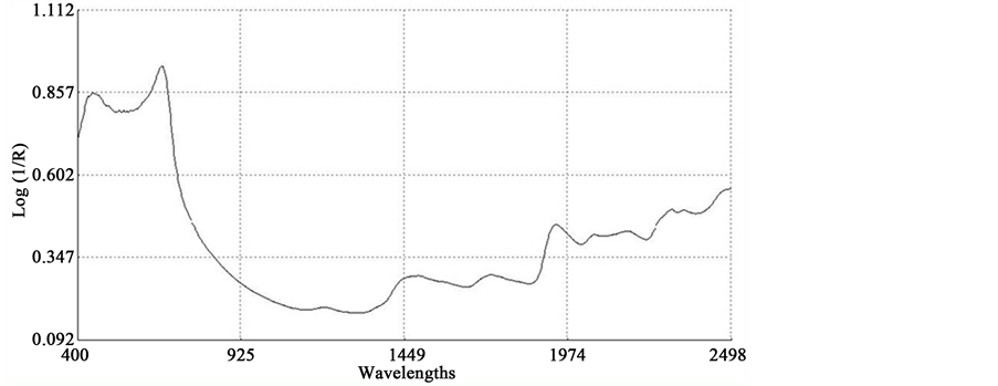
An average raw NIR reflectance spectrum of the samples is shown in Figure 1(a). The second derivative was calculated from the log(1/R) spectra at gaps of 4 data points (8 nm) and a smoothing over segments of 4 data points (2,4,4,1) with scatter correction (SNVD). The derivative form of an average spectrum is shown in Figure 1(b).
In the average raw spectrum (Figure 1(a)), the main absorption bands were observed over several wavelengths such as 1436-1464, 1720, 1926, 2100 - 2136, 2302 - 2344, and 2488 nm. The overlaid raw spectra for all 120 samples shown in Figure 2 reflect the fact that they belong to same population despite they were for various plant parts of two different species. The second-derivative spectra generally show a trough corresponding to each peak in the original spectra, removing the overlapping peaks and baseline effects [53] . The chemical interpretations with regards to various functional groups responsible for absorption/re- flection of NIR radiation at various wavelengths have been described by Workman and Weyer [54] . The second derivative of an average spectrum (Figure 1(b)) showed absorption bands at 1398 nm related to C-H bands of methylene
 (a)
(a)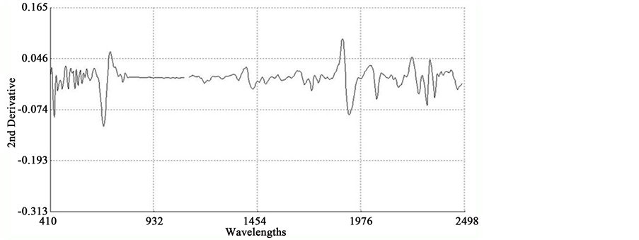 (b)
(b)
Figure 1. Raw spectrum (log 1/R; (a) and second derivative (2,4,4,1 + SNVD; (b) of NIRS average spectrum of a sunflower/soybean plant sample.
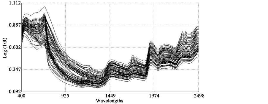
Figure 2. Overlaid raw spectra (log 1/R) of all 120 sunflower and soybean plant samples.
(-CH2) group associated with aliphatic and aromatic hydrocarbons; 1454 nm related to O-H stretching first overtone of starch, C-H bending of methylene (-CH2) of hydrocarbons and O-H stretching of starch; 1480 nm related to N-H stretching first overtone of -NH2C=O; 1526 nm related to N-H stretching first overtone of -NH2R; and 1742 nm related to S-H stretching first overtone of thiol group associated with thiols. The bands at 1780 nm was related to C-H stretching first overtone of cellulose and H-O-H deformation and bending of cellulose, 1794 nm was related to O-H bending of water, 1962 nm was related to O-H stretching and O-H bending combination band of starch, 2099 nm was related to O-H bending or C-O stretching third overtone of starch or cellulose, 2186 nm was related to N-H bending second overtone of protein, C-H stretching or C=O bending of protein, 2280 and 2348 nm were related to C-H stretching or -CH2 deformation-bending of starch, and 2304 nm was related to C-H bending second overtone of protein.
As an analytical method, the NIRS is based on the magnitude of absorption/reflection of NIR radiation at a specific wavelength or within a specific region of wavelength by the samples of various natural products. The assignment of main absorption bands in the second derivative of an average spectrum to various probable functional groups, as described above, was done according to literature compiled by Workman and Weyer [55] , which showed a good agreement with the information for the functional groups in the spectrum given by WinISI software. The wavelength specific absorption/reflection of NIR radiation usually depends on the presence and abundance of some specific functional groups of various organic compounds in the samples. However, it is often difficult to accurately determine what wavelength(s) or region(s) in the near-infrared spectrum carried the most quantitative information about the contents of natural compounds being analyzed even though the NIRS technique works fairly well in many cases. It also evident in the literature that the chemical interpretation for absorption/reflection of NIR radiation, at a specific wavelength, often varies according to what experimental materials and chemical components are being considered NIR analysis [41] [55] [56] . Nevertheless, the NIRS technique has successfully been employed for determining the contents of various natural compounds in food, feed, biomass, and other natural products even without pinpointing chemical information regarding prominent functional groups related to the near-infrared spectrum [32] [44] [50] [55] [56] [57] [58] [59] .
3.3. Calibration Models: Effect of Various Mathematical Treatments
Initially, nine different math treatments (0,4,4,1; 1,4,4,1; 2,4,4,1; 0,5,5,1; 1,5,5,1; 2,5,5,1; 0,10,5,1; 1,10,5,1; and 2,10,5,1) were used to develop calibration models for each of the 27 different parameters leading to a total of 243 models. The accuracy of each of these calibration models was evaluated based on the coefficients of determination (R2) for predicted versus measured compositions in calibration phase and the ratio of standard deviation of data set (SD) to standard error of cross validation (SECV), RPDc.
According to Williams [60] , a value for R2 between 0.50 and 0.65 indicates that more than 50% of the variance in Y is accounted for by variance in X, so that discrimination between high and low concentrations can be made (qualitative prediction); a value for R2 between 0.66 and 0.81 indicates “approximate” quantitative predictions, whereas, a value for R2 between 0.82 and 0.90 reveals “good” prediction; calibration models having a value for r2 above 0.91 are considered to be “excellent”. The RPDc is the factor by which the prediction accuracy has been increased compared to using the mean composition for all samples in the calibration set. A wide variety of interpretations of RPDc values to indicate the quality of calibrations are found in the literature [38] [43] [47] [60] [61] [62] [63] [64] . Williams [60] suggested five levels of prediction accuracy based on RPDc values: (1) a value for the RPDc below 1.5 indicates that the calibration is not usable; (2) a value between 1.5 and 2.0 reveals a possibility to distinguish between high and low values; (3) a value between 2.0 and 2.5 makes “approximate” quantitative prediction; (4) a value between 2.5 and 3.0 suggests “good” quantitative prediction; and (5) a value greater than 3.0 indicates “excellent” quantitative prediction. Using both R2 and RPDc, we categorized the 243 calibration models according to two different categorization schemes as follows:
Categorization Scheme 1
Excellent: R2 > 0.90 and RPDc > 3; Good: 0.81 < R2 < 0.90 and 2.5 < RPDc < 3; Approximate: 0.66 < R2 < 0.80and 2.0 < RPDc < 2.5; and Poor: R2 < 0.66 and RPDc < 2.0, according to Saeys et al. [38] and Zornoza et al. [62] .
Categorization Scheme 2
Category A: RPDc > 2.0 and R2 > 0.80; Category B: RPDc, 1.4 - 2.0 and R2, 0.50 - 0.80; and Category C: RDPc < 1.4 and R2 < 0.50, according to Chang et al. [42] .
Use of underivatized raw spectra (for example, 0,4,4,1 math treatment) generally gave inferior quality calibration models as compared to when first (for example, 1,4,4,1) and second (for example, 2,4,4,1) derivatives of the raw spectra were used in calibration development (Table 3). According to the categorization
Table 3. Effects of various math treatments on the distribution of 27 NIRS calibration models of sunflower and soybean plant samples under various categories.
Scheme 1, the math treatment 2,4,4,1 generally resulted in more improved distribution of the 27 calibration models than any other math treatments. However, this math treatment yielded “poor” calibration models for starch and ESC, whereas an “approximate” quantitative model for ESC was obtained by applying 1,4,4,1 math treatment. In contrast, with the categorization Scheme 2, the math treatment 1,4,4,1 placed higher number of calibration models in category-A than 2,4,4,1. There was no change in such distribution with 1,5,5,1 versus 2,5,5,1 math treatments and a slight change with 1,10,5,1 versus 2,10,5,1 math treatments. The categorization Scheme 1 is more comprehensive than the Scheme 2. There- fore, only the calibrations developed using 2,4,4,1 math treatment were further evaluated using the independent validation set. None of the math treatments produced an acceptable calibration model for starch.
Table 4 depicts the calibration and cross validation statistics such as coefficient determinations (R2 and 1-VR) and standard errors (SEC and SECV) along with the RPDc for a selected set of models developed using different math treat- ments.
Table 4. Effects of various math treatments on some important NIRS calibration development statistics for some selected parameters of sunflower and soybean plant samplesa.
aThe math treatments that used underivatized raw spectra (0,4,4,1; 0,5,5,1; and 0,10,5,1) have been omitted because of their inferior performance.
3.4. The Calibration Models Given by 2,4,4,1 Math Treatment
As discussed in section 3.3, further evaluations of the models were kept limited with in-depth examination of the calibration and cross validation statistics given by the math treatment 2,4,4,1 because this option gave better calibration models for the highest number of constituents (out of 27 total). The calibrations and cross validations statistics of the NIRS models developed by this option for all 27 constituents of sunflower and soybean plant samples are shown in Table 5. We also observed that the use of the whole visible-NIR range (400 - 2498 nm) resulted in much higher R2 and 1-VR and lower SEC and SECV than when using either just the visible range (400 - 1100 nm) or just the near-infrared range (1100 - 2498 nm) (data not shown). Optimum wavelengths for NIR analysis mostly rely on empirical calibrations for predicting qualitative constituents in agricultural products. This is because of the broad array of chemical compounds present in the samples, which lead to overlapping and perturbed NIR absorption bands [41] .
Generally, except for starch and simple sugars (ESC), the calibration models for the other 25 parameters had good quantitative information. These models had low standard error of both calibration (SEC) and cross validation (SECV) with high coefficient of determination in both calibration (R2 = 0.6993 - 0.9986) and cross validation (1-VR = 0.5377 - 0.9966). According to the categorization Scheme 1, as many as 18 of these models were found to be “excellent” with R2 > 0.90 and RPDc > 3.0, these included moisture, DM, CP, fat, ash, lignin, NFC, WSC, NSC, Ca, P, total-N, S, Al, Cu, Fe, Mn, and Zn. The models for B and K were “good” with 0.80 < R2 ≤ 0.90 and 2.5 < RPDc ≤ 3.0, and the 5 models for
Table 5. Equation development statistics using MPLS and scatter correction (2,4,4,1 SNVD) for the NIRS prediction of the 27 constituents of sunflower and soybean plant samples.
aSamples used to develop the model. bNumber of PLS loading factors in the regression model MPLS (modified partial least-squares). cSEC, standard error of calibration. dR2, coefficient of determination of calibration. e1 − Vr, one minus the ratio of unexplained variance divided by variance. fSECV, standard error of cross-validation. gRPDc, SD/SECV, the ratio of standard error of cross validation to deviation (SD, standard deviation of reference data in calibration set). hRPIQc, IQ/SECV, the ratio of standard error of cross validation to inter-quartile distance (IQ, inter-quartile distance in reference data in the calibration set). iE: Excellent (r2 > 0.90 and RPD > 3), G: Good (0.81 < r2 < 0.90 and 2.5 < RPD < 3), A: Approximate: (0.66 < r2 < 0.80 and 2.0 < RPD < 2.5), P: Poor (r2 < 0.66 and RPD < 2).
ADF, NDF, cellulose, hemicellulose, and Mg were “approximate” with 0.65 < R2 ≤ 0.80 and 2.0 < RPDc ≤ 2.5. The calibration models for starch and ESC were “poor” with R2 < 0.65 and RPDc < 2.0. The low R2 and RPDc for ADF, NDF, cellulose, and hemicelluloses may be due to their negative correlation with the oil and protein content as well as the NIR absorption characteristics of their hemicellulose and cellulose fractions [50] [65] [66] [67] .
The same 27 models were also grouped into three categories (A, B, and C) according to the Scheme 2, but the details of this exercise are not shown for the sake of brevity except for the summary reported in Table 3. The Category A (RPD > 2.0) includes 21 constituents (Table 3) with measured versus predicted R2 values between 0.80 and 1.00. These constituents are fat, CP, N, Ash, Ca, S, Fe, Al, WSC, NFC, Mn, Zn, P, NSC, Cu, lignin, DM, moisture, K, B, and cellulose. Such results indicate that these constituents were readily and accurately predicted [42] . Category B (RPD =1.4 - 2.0) includes constituents with measured versus predicted R2 values between 0.50 and 0.80. This group includes 4 constituents namely ADF, NDF, hemicellulose, and Mg. Starch and ESC (simple sugars) are in Category C (R2 < 0.50, RPD < 1.4). Chang et al. [42] suggested that prediction of constituents in Category B can be improved by using different calibration strategies, but the constituents in Category C may not be reliably predicted using NIRS at all. However, in our study we found that the prediction of ESC improved from Category C in 2,4,4,1 math treatment (R2 = 0.4964, RPD = 1.41) to Category A in 1,4,4,1 math treatment (R2 = 0.8380, RPD = 2.48) in addition to improvement of NDF prediction from Category B in 2,4,4,1 math treatment (R2 = 0.7973, RPD = 2.22) to Category A in 1,4,4,1 math treatment (R2 = 0.8441, RPD = 2.53).
Asekova et al. [50] developed NIRS calibration of soybean forage quality and reported R2 and RPD values of 0.934 and 3.85 for crude fiber (CF), 0.909 and 3.25 for CP, 0.767 and 2.07 for NDF, and 0.748 and 1.97 for ADF. With whole plant biomass of sunflower, the NIRS calibration models reported by Fassio et al. [49] had R2 and RPD values of 0.82 and 2.0 for DM, 0.86 and 2.9 for CP, 0.85 and 2.2 for ash, 0.62 and 1.2 for NDF, 0.64 and 1.8 for ADF, and 0.50 and 1.2 for hemicellulose.
The RPIQc (IQ/SECV) is another such criterion, which has been claimed to be a more robust one than RPDc because it is based on inter-quartile distance instead of SD, which better represents the spread of the population [45] . The calculated values of RPIQc were >3.0 for 23 constituents, between 2.5 - 3.0 for Mg, between 2.0 - 2.5 for ADF, and <2.0 for starch and ESC, reconfirming the high accuracy of at least 23 out of 27 models. However, the original paper of Bellon-Maurel et al. [45] , where the RPIQc was proposed as a judging criterion of NIRS calibration model, did not discuss the interpretation of the situation having a high RPIQc but a relatively low RPDc as observed for ADF, NDF, cellulose, hemicellulose calibrations of this study. Therefore, the acceptance or rejection of a calibration model solely based on RPIQc or RPDc value remains questionable. The other judging criteria (such as R2, SEC, and SECV) must be taken into consideration. Based on this trend, a few of the 27 models that have been categorized as “Approximate”, leaving room for further improvement, but should not be considered as failed, because they yielded acceptable values of all other statistics used in numerous reports as the judging criteria for NIRS calibration models. In this context, we suggest that the independent validation performance should be closely monitored and could be used as the judging criteria with even more emphasis.
Figure 3 shows the plots of laboratory reference values versus NIR predicted values for a selected set of 6 constituents such as DM, CP, ADF, NDF, lignin, and P contents for the calibration set. Such plots for the remaining 21 constituents are not shown for the sake of brevity. The diagonal dashed line in each plot is the 1:1 line. The closeness of the plotted data points to this line indicates the closeness between the NIR predicted values and the corresponding laboratory reference values. The results indicate the slopes of the measured versus predicted regression lines for these 6 constituents are not significantly different from 1.00, the slope was even exactly 1.00 for DM, ADF, NDF. This observation when considered alone may suggest that NIRS-MPLS did not tend to significantly over- or underestimate all of these 6 constituents. But other criteria need to be evaluated before reaching such a conclusion. For example, the model of ADF was categorized as “Category-B” and “approximate” by the two categorization schemes used; despite this, the model for ADF yielded a slope of 1.00 for the measured vs. predicted regression line. Given the fact that this model had higher SECV and lower 1-VR, the plot is showing greater scatter around the 1:1 line. So a slope of 1.00 alone is not a good indicator of how well the data are predicted. Likewise, the interpretation of the two categorization schemes merits reconsideration case by case. As revealed in the plots for DM, the values deviate from normal to some extent with higher frequency of the lower values. Such a high density of low values often results in more favorable coefficients of determination than when the values are more evenly distributed over the range. Inclusion of some samples with DM content higher than 90% may impart further robustness to the model developed.
In this study, we attempted to develop NIRS calibration models for 11 different minerals such as Ca, K, Mg, P, S, Al, B, Cu, Fe, Mn, and Zn contents of sunflower and soybean plant samples. The results show that VIS-NIRS-MPLS produced “excellent (r2 > 0.90 and RPDc > 3.0)” quantitative calibration models for Ca, P, S, Al, Cu, Fe, Mn, and Zn (8 in total), “good (0.80 < r2 ≤ 0.90 and 2.5 < RPDc ≤ 3.0)” calibration models for K and B, and “approximate (0.65 < r2 ≤ 0.80 and 2.0 < RPDc ≤ 2.5)” calibration model for Mg. Given the narrow range of plant mineral contents, some authors, however, recommended that NIRS calibration models for minerals should be evaluated by coefficient of variation (CV) or RPDc instead of coefficient of determination (R2) [68] .
Analysis of mineral concentration with NIRS produces mixed results since minerals per se do not absorb visible (VIS) or NIR light and their concentrations are low in typical plant tissues. However, their detection by VIS-NIR spectros-
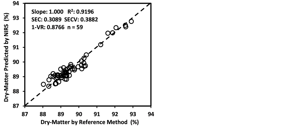
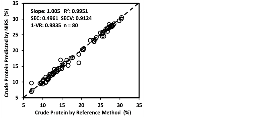
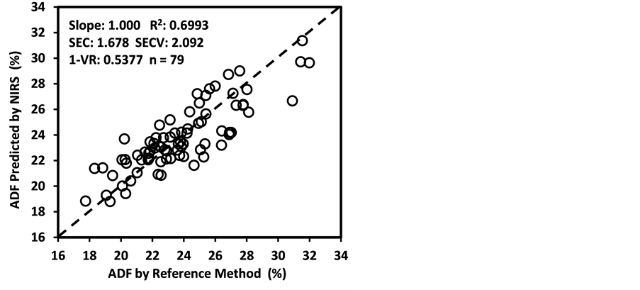
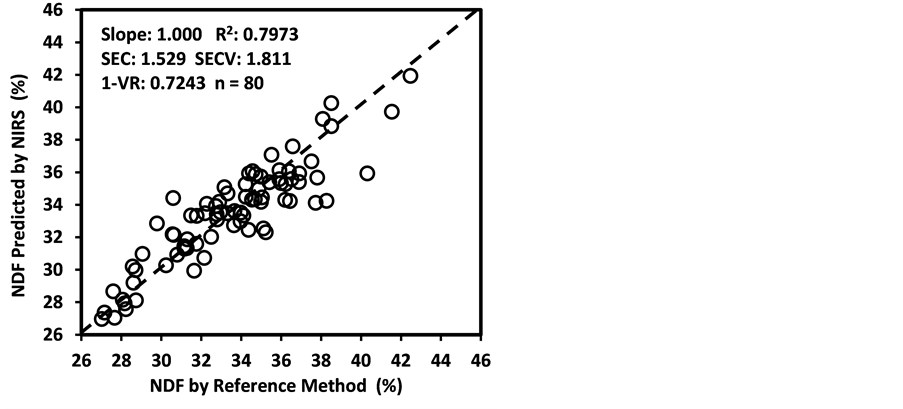
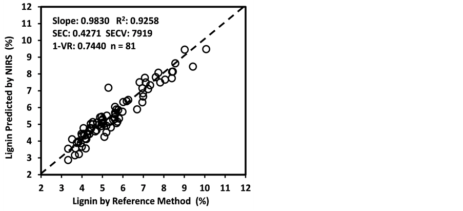
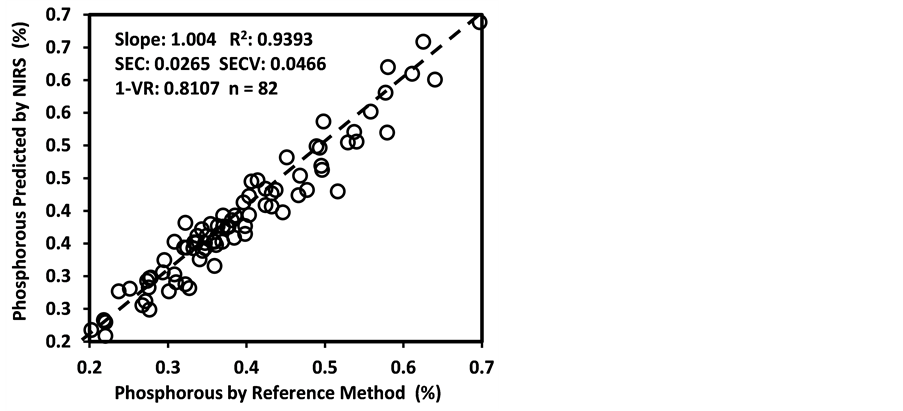
Figure 3. Scatter plots of NIRS predicted values versus laboratory reference values for calibration sets of some selected parameters of sunflower and soybean plant samples.
copy has been possible because minerals exist in plant tissue as complexes formed with various NIR-active organic compounds; the concentrations of many of such compounds vary both among and within species [69] . For example, in plants with both P deficiency and sufficiency, existence of plant P predominantly in the form of NIR-active P compounds in plants such as phytates, phospholipids and nucleic acids [70] [71] supports the development of sound NIRS calibration of plant-P. However, excessive uptake of P often increases the accumulation of metabolically inactive inorganic P [71] resulting in relatively poor performance of P calibrations as observed in other studies [47] [72] [73] . The calibration of N typically utilizes the correlation between N and chlorophyll. Further inclusion of the signal from N-H and peptide bonds of proteins indicates a more solid correlation to N concentrations [67] [74] . In this study, the Mg content yielded only an “approximate” calibration model despite the fact that Mg is the central element in chlorophyll, its calibration frequently relies on the strong chlorophyll signal in the VIS-NIR region [74] [75] . However, partitioning of total plant Mg and chlorophyll-bound Mg is more important in this context, which is highly variable for Mg-sufficient versus Mg-deficient plants. In a Mg-sufficient plant, less than 6% of the Mg content may be bound in chlorophyll. In Mg-deficient plant this proportion can increase up to 35%, and in combination with low light conditions, which increase chlorophyll concentrations, more than 50% of the total plant Mg may be bound in chlorophyll [71] . Such variability in the distribution of total plant Mg and chlorophyll-bound Mg may often hinder the success of achieving good VIS-NIRS calibration of Mg as observed in this study. Beside N and Mg deficiency, numerous other factors may also affect the chlorophyll concentration, as demonstrated by Ward et al. [47] . A good number of earlier studies generally obtained poor or at most “qualitative” NIRS calibrations [64] [76] for Fe, Mn, Zn, Cu, and B. In contrast, we obtained “excellent (r2 > 0.90 and RPDc > 3.0)” or “good (0.80 < r2 ≤ 0.90 and 2.5 < RPDc ≤ 3.0)” quantitative calibration models for Ca, S, Al, Cu, Fe, Mn, Zn, K, and B as reported by Menesatti [71] for Fe, Mn, and Zn.
3.5. Independent Validation of the Calibration Models
The predictability of the all 27 NIRS calibration models developed using 2,4,4,1 math treatment was tested through a validation exercise carried out with a set of samples independent of the calibration set. The number of samples included in the validation set varied from 28 - 35 for different constituents, which were about half of the number of samples included in the corresponding calibration set.
The statistics of such external validation exercise such as r2, bias, bias (limit) (maximum allowable bias), SEP, SEPc (the bias-corrected SEP), SEPc (limit) (the maximum allowable SEPc), slope, RPDv (SD/SEP), and RPIQv (IQ/SEP) values for the models are presented in Table 6. These statistics were utilized to evaluate the predictability or reliability of the calibration models. An NIRS calibration model is considered robust and reliable when it can produce lower bias [(lower
Table 6. Monitoring (external validation) statistics for the NIRS prediction equations developed with 2,4,4,1 math treatment for the 27 constituents of sunflower and soybean plant samples.
aSamples (independent) used to monitor the model. bSD, standard deviation of mean. cIQ, inter-quartile distance (IQ, inter-quartile distance in reference data). dBias, average difference between reference and NIRS values. eBias(limit) maximum allowable value of bias.fr2, coefficient of determination in external validation. gSEP, standard error of prediction. hSEPc, the bias-corrected standard error of prediction. iSEPc(limit), the maximum allowable value of SEPc. jSlope and intercept, the steepness and intercept of a straight line curve for the plot between the NIR predicted values versus reference values. kRPD, SD/SEP, the ratio of performance to deviation (SEP to the SD of the reference data in the external validation set). lRPIQ, IQ/SEP, the ratio of performance to inter-quartile distance (SEP to the IQ of the reference data in the external validation set). mE: Excellent (r2 > 0.90 and RPD > 3), G: Good (0.81 < r2 < 0.90 and 2.5 < RPD < 3), A: Approximate: (0.66 < r2 < 0.80 and 2.0 < RPD < 2.5), P: Poor (r2 < 0.66 and RPD < 2).
than the bias(limit)] and SEPc [(lower than the SEPc (limit)] with r2 and slope close to 1.0, and RPDv and/or RPIQv values greater than 2.0 in external validation with samples independent of calibration sample set [42] [43] [45] [46] . In general, the slope, r2 and RPDv values obtained during external validation for all models except starch were high enough to indicate good agreement between reference values and NIRS predicted values (slope > 0.90; r2 > 0.80; and RPDv > 2.0) (Table 6), similar in most cases to the corresponding statistics obtained during the calibration development (Table 5). Figure 4 depicts the plots of NIRS predicted values versus laboratory reference values in the validation set for DM, CP, ADF, NDF, lignin, and P contents, which shows the significant relationship between NIRS predicted values and laboratory reference values.
As depicted in Table 6, the validation performance was “excellent” (r2 > 0.90 and RPDv > 3.0) for 23, “good” (0.81 < r2 < 0.90 and 2.5 < RPDv < 3) for 1, “approximate” (0.66 < r2 < 0.80 and 2.0 < RPDv < 2.5) for 2, and “poor” (r2 < 0.66 and RPDv < 2.0) for 1 models according to the categorization Scheme 1 [44] [62] . In contrast, the calibration performance of these models was “excellent” (R2 > 0.90 and RPDc > 3.0) for 18, “good” (0.81 < R2 < 0.90 and 2.5 < RPDc < 3.0) for 2, “approximate” (0.66 < R2 < 0.80 and 2.0 < RPDc < 2.5) for 5, and “poor” (R2 < 0.66 and RPDc < 2.0) for 2 models (Table 3). That means actual predictability of some models was better than what was expected based on their calibration statistics. For example, despite the models for ADF, cellulose, hemicellulose, WSC, ESC, and Mg were “approximate” (0.66 < R2 < 0.80 and 2.0 < RPDc < 2.5) based on calibration performance, they were “excellent” (r2 > 0.90 and RPDv > 3.0) or “good” (0.81 < r2 < 0.90 and 2.5 < RPDv < 3.0) based their validation performance, suggesting that these models are also reliable for quantitative prediction. Likewise, the model for ESC was “poor” (R2 < 0.66 and RPDc < 2.0) based on calibration performance, but it was able to offer an “approximate” prediction during a validation exercise. Thus, the schemes for categorizing NIRS calibration models available in the literature should be carefully used for judging the quality of the models. We suggest putting more emphasis on the performance criteria of independent validation in judging the quality of the model.
4. Conclusions
Soybean and sunflower have the potential to be used as forage crops in addition to their traditional use as protein and/or oil yielding crops. In integrated forage-based livestock production industries, high throughput in analysis is important for evaluating forage quality and diagnosing and correcting forage nutrient deficiency. NIRS method is especially suitable in such case because it replaces the time consuming wet-chemistry methods without sacrificing accuracy and precision.
This study demonstrated that composition of various plant parts of both soybean and sunflower could be calibrated as a single population covering multiple sampling dates and under varying tillage treatments, which is very useful but contrary to common belief. Except starch, the NIRS calibration models for all
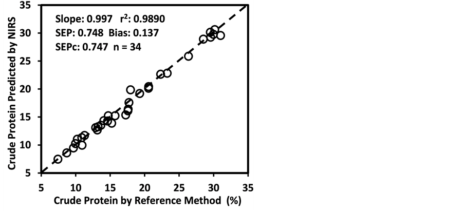
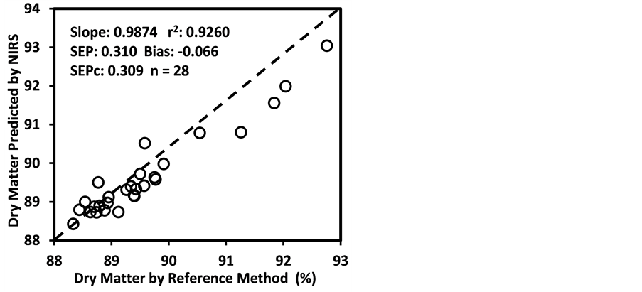
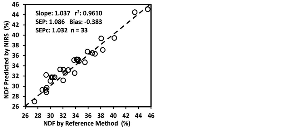
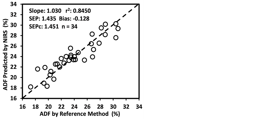
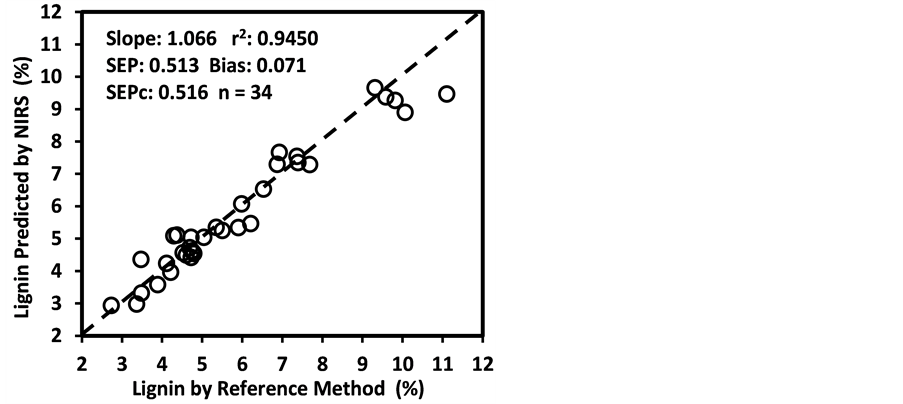
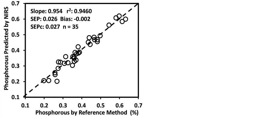
Figure 4. Scatter plots of NIRS predicted values versus laboratory reference values for external validation sets of some selected parameters of sunflower and soybean plant samples.
other 26 forage quality parameters showed good results with 24 models ranging from good to excellent in their quantitative predictability. These models can be reliably applied in the routine analysis of soybean and sunflower forage quality for the purposes of livestock nutrient management decisions. The study also showed NIRS as a reliable analytical tool for decision making allowing determination of multiple values in a single analytical procedure thereby assisting in timely decision making for efficient nutrient management for livestock. Although development of an NIRS laboratory entails significant initial start-up costs, it is relatively inexpensive in the long term. It is also considered as “cheap” and “green chemistry” because it does not involve any chemicals and does not generate any hazardous wastes. However, the problem of spectral outliers should be watched and solved by updating, expanding, and improving the initially developed and validated calibrations by including future samples from different environments and species and covering a wider range of the parameters. This will impart further robustness to the current calibration models. Nonetheless, the results accomplished in this study would contribute to expand organic production system including soybean and sunflower particularly in the southern United States.
Acknowledgements
The authors duly acknowledge the funding received through a Sustainable Agricultural Research and Education Grant Project Number LS10-232 (http://www.sare.org).
Disclaimer
This publication is a joint contribution of the Agricultural and Environmental Services Laboratories, University of Georgia, Athens, GA, and the US Department of Agriculture, Agricultural Research Service, (ARS) Southeast Watershed Research Laboratory and Crop Protection and Management Research Laboratory, Tifton, GA. The use of trade, firm, or corporate names in this publication is for the information and convenience of the reader and does not constitute an official endorsement or approval by the University of Georgia or the US Department of Agriculture, Agricultural Research Service of any product or service to the exclusion of others that may be suitable.
Cite this paper
Saha, U., Endale, D., Tillman, P.G., Johnson, W.C., Gaskin, J., Sonon, L., Schomberg, H. and Yang, Y.G. (2017) Analysis of Various Quality Attributes of Sunflower and Soybean Plants by Near Infrared Reflectance Spectroscopy: Development and Validation Calibration Mo- dels. American Journal of Analytical Chemistry, 8, 462-492. https://doi.org/10.4236/ajac.2017.87035
References
- 1. Acikgoz, E., Sincik, M., Karasu, A., Tongel, O., Wietgrefe, G., Bilgili, U., Oz, M., Albayarak, S., Turan, Z.M. and Goksoy, A.T. (2009) Forage Soybean Production for Seed in Mediterranean Environments. Field Crops Research, 110, 213-218.
- 2. Devine, T.E. and McMurtrey III, J.E. (2004) Registration of “Tara” Soybean. Crop Science, 44, 1020-1021.
https://doi.org/10.2135/cropsci2004.1020 - 3. Asekova, S., Shannon, J.G. and Lee, J.D. (2014) The Current Status of Forage Soybean. Plant Breeding and Biotechnology, 2, 334-341.
https://doi.org/10.9787/PBB.2014.2.4.334 - 4. Orozco, L.R., Castro-Alegria, A. and Fievez, V. (2013) Ensiled Sorghum and Soybean as Ruminant Feed in the Tropics, with Emphasis on Cuba. Grass and Forage Science, 68, 20-32.
https://doi.org/10.1111/j.1365-2494.2012.00890.x - 5. Chang, S.R., Lu, C.-H., Lur, H.-S. and Hsu, F.-H. (2012) Forage Yield, Chemical Contents, and Silage Quality of Manure Soybean. Agronomy Journal, 104, 130-136.
https://doi.org/10.2134/agronj2011.0015 - 6. Sheaffer, C.C., Orf, J.H., Devine, T.E. and Jewett, J.G. (2001) Yield and Quality of Forage Soybean. Agronomy Journal, 93, 99-106.
https://doi.org/10.2134/agronj2001.93199x - 7. Nielsen, D.C. (2011) Forage Soybean Yield and Quality Response to Water Use. Field Crops Research, 124, 400-407.
- 8. NDSU Extension Service (2007) Sunflower Production. Bulletin A-1331 (EB-25 Revised). North Dakota Agricultural Experiment Station and North Dakota State University Extension Service, Fargo, ND.
- 9. McClure, M.A., Allen, F.L., Johnson, R.D. and Heatherly, L.G. (2010) Sunflower: An Alternative Crop for Tennessee Producers. Production Guidelines and Tennessee Hybrid Trials. Bulletin SP721, The University of Tennessee Institute of Agriculture, Knoxville, TN.
- 10. NSA (National Sunflower Association) (2017) 2016 U.S. Sunflower Crop Quality Report. National Sunflower Association, Mandan, ND.
- 11. Mafakher, E., Meskarbashee, M., Hassibi, P. and Mashayekhi, M.R. (2010) Evaluation of Sunflower Silage in Development Stages. Asian Journal of Crop Science, 2, 20-24.
https://doi.org/10.3923/ajcs.2010.20.24 - 12. Kansas Forage Task Force (2017) Sunflower Silage. Forage Facts Series Fora31. Kansas State University Agricultural Experiment Station and Cooperative Extension Service.
https://www.asi.K-state.edu/doc/forage/fora31.pdf - 13. Shenk, J.S., Westerhaus, M.O. and Hoover, M.R. (1979) Analysis of Forage by Near Infrared Reflectance. Journal of Dairy Science, 62, 807-812.
https://doi.org/10.3168/jds.S0022-0302(79)83330-5 - 14. AOAC (1996) Moisture in Animal Feed, Method 930.15. 16th Edition, Official Methods of Analysis of AOAC International, Gaithersburg, MD.
- 15. Etheridge, R.D., Pesti, G.M. and Foster, E.H. (1998) A Comparison of Nitrogen Values Obtained Utilizing the Kjeldahl Nitrogen and Dumas Combustion Methodologies (Leco CNS 2000) on Samples Typical of an Animal Nutrition Analytical Laboratory. Animal Feed Science and Technology, 73, 21-28.
https://doi.org/10.1016/S0377-8401(98)00136-9 - 16. Kirsten, W.J. (1979) Automated Methods for the Simultaneous Determination of Carbon, Hydrogen, Nitrogen and Sulfur, and Sulfur Alone in Organic and Inorganic Materials. Analytical Chemistry, 51, 1173-1179.
https://doi.org/10.1021/ac50044a019 - 17. Dumas, J.B.A. (1831) Procedes de l’analyse Organic. Annales de Chimie et de Physique (Annals of Chemistry and of Physics), 247, 198-213.
- 18. ASTM Standards D3174-97 (1998) Standard Test Method for Ash in the Analysis Sample of Coal and Coke, Section 5, Vol. 05.05, Annual Book of ASTM Standards, ASTM International, West Conshohocken, PA, 303-305.
- 19. ANKOM Technology (2006) Neutral Detergent Fiber in Feeds-Filter Bag Technique, Method 6, ANKOM Technology.
http://www.ankom.com/media/documents/NDF_081606_A200.pdf - 20. ANKOM Technology (2006) Acid Detergent Fiber in Feeds Filter Bag Technique, Method 5, ANKOM Technology.
http://www.ankom.com/media/documents/ADF_81606_A200.pdf - 21. Undersander, D., Martens, D.R. and Thiex, N. (1993) National Forage Testing Association, Method 5.1: Determination of Amylase Neutral Detergent Fiber by Refluxing, Forage Analysis Procedures, National Forage Testing Association.
http://www.foragetesting.org/index.php?page=lab_procedures - 22. Undersander, D., Martens, D.R. and Thiex, N. (1993) National Forage Testing Association, Method 4.1: Determination of Acid Detergent Fiber by Refluxing, Forage Analysis Procedures, National Forage Testing Association.
http://www.foragetesting.org/index.php?page=lab_procedures - 23. ANKOM Technology (2005) Method for Determining Acid Detergent Lignin in Beakers, Method 08/05, ANKOM Technology Method 08/05.
http://www.ankom.com/media/documents/ADL_beakers.pdf - 24. Karkalas, J.J. (1985) An Improved Enzymatic Method for the Determination of Native and Modified Starch. Journal of the Science of Food and Agriculture, 36, 1019-1027.
https://doi.org/10.1002/jsfa.2740361018 - 25. Holm, J., Bjorck, I., Drews, A. and Asp, N.G. (1986) A Rapid Method for the Analysis of Starch. Starch/Starke, 38, 224-226. https://doi.org/10.1002/star.19860380704
- 26. Smith, D. (1969) Removing and Analyzing Total Nonstructural Carbohydrates from Plant Tissue. Research Report No. 41, Wisconsin Agricultural Experiment Station.
- 27. Dubois, M., Gilles, K.A., Hamilton, J.K., Roberts, P.A. and Smith, F. (1956) Colorimetric Method for Determination of Sugars and Related Substances. Analytical Chemistry, 28, 350-356.
https://doi.org/10.1021/ac60111a017 - 28. Harris Jr., B. (2003) Nonstructural and Structural Carbohydrates in Dairy Cattle Rations, Extension Circular 1122. University of Florida, IFAS.
- 29. USEPA (1995) Microwave Assisted Acid Digestion of Siliceous and Organically Based Matrices, Method 3052. 3rd Edition, Test Methods for Evaluating Solid Waste, US Environmental Protection Agency, Washington DC.
- 30. Creed, J.T., Brockhoff, C.A. and Martin, T.D. (1994) Determination of Trace Elements in Waters and Wastes by Inductively Coupled Plasma-Mass Spectrometry, US-EPA Method 200.8, Revision 5.4 EMMC Version. Environmental Monitoring Systems Laboratory, Office of Research and Development, Revision 5.4 EMMC Version, U.S. Environmental Protection Agency, Cincinnati, OH.
- 31. Rushing, J.B., Saha, U.K., Lemus, R., Sonon, L. and Baldwin, B.S. (2016) Analysis of Some Important Forage Quality Attributes of Southeastern Wildrye (Elymus glabriflorus) Using Near-Infrared Reflectance Spectroscopy. American Journal of Ana- lytical Chemistry, 7, 642-662.
- 32. Shenk, J.S. and Westerhaus, M.O. (1995) Analysis of Agriculture and Food Products by Near Infrared Reflectance Spectroscopy. Monograph, NIR Systems, Silver Spring, MD.
- 33. Shenk, J.S. and Westerhaus, M.O. (1991) Population Definition, Sample Selection and Calibration Procedures for Near Infrared Reflectance Spectroscopy. Crop Science, 31, 469-474. https://doi.org/10.2135/cropsci1991.0011183X003100020049x
- 34. Windham, W.R., Mertens, D.R. and Barton, F.E. (1989) Protocol for NIRS Calibration: Sample Selection and Equation Development and Validation. In: Marten, G.C., Ed., Near Infrared Reflectance Spectroscopy (NIRS): Analysis of Forage Quality, USDA Agricultural Handbook, Washington DC, 643.
- 35. Windham, W.R., Fales, S.L. and Hoveland, C.S. (1988) Analysis for Tannin Concentration in Sericea lespedeza by Near IR Reflectance Spectroscopy. Crop Science, 28, 705-708. https://doi.org/10.2135/cropsci1988.0011183X002800040031x
- 36. Shenk, J.S. and Westerhaus, M.O. (1996) Calibration the ISI Way. In: Davis, A.M.C. and Williams, P., Eds., Near Infrared Spectroscopy: The Future Waves, NIR Publications, Chichester, 198-202.
- 37. Lestander, T.A. and Christofer, R. (2005) Multivariate NIR Spectroscopy Models for Moisture, Ash and Calorific Content in Biofuels Using Bi-Orthogonal Partial Least Squares Regression. Analyst, 130, 1182-1189.
- 38. Saeys, W., Mouazen, A.M. and Ramon, H. (2005) Potential for Onsite and Online Analysis of Pig Manure Using Visible and Near Infrared Reflectance Spectroscopy. Biosystem Engineering, 91, 393-402.
- 39. Barnes, R.J., Dhanoa, M.S. and Lister, S.J. (1989) Standard Normal Variate Transformation and De-Trending of Near-Infrared Diffuse Reflectance Spectra. Applied Spectroscopy, 43, 772-777.
https://doi.org/10.1366/0003702894202201 - 40. Shenk, J.S. and Westerhaus, M.O. (1991) Population Structuring of Near Infrared Spectra and Modified Partial Least Squares Regression. Crop Science, 31, 1548-1555.
https://doi.org/10.2135/cropsci1991.0011183X003100060034x - 41. Kim, K.S., Park, S.H. and Choung, M.G. (2007) Nondestructive Determination of Oil Content and Fatty Acid Composition in Perilla Seeds by Near-Infrared Spectroscopy. Journal of Agriculture and Food Chemistry, 55, 1679-1685.
https://doi.org/10.1021/jf0631070 - 42. Chang, C.W., Laird, D.A., Mausbach, M.A. and Hurburgh Jr., C.R. (2001) Near-Infrared Reflectance Spectroscopy-Principal Components Regression Analyses of Soil Properties. Soil Science Society of America Journal, 65, 480-490.
https://doi.org/10.2136/sssaj2001.652480x - 43. Reeves III, J.B. (2001) Near-Infrared Diffuse Reflectance Spectroscopy for the Analysis of Poultry Manures. Journal of Agriculture and Food Chemistry, 49, 2193-2197.
https://doi.org/10.1021/jf0013961 - 44. Mowrer, J., Kissel, D., Cabrera, M. and Hassan, S. (2014) Near-Infrared Calibrations for Organic, Inorganic, and Mineralized Nitrogen from Poultry Litter. Soil Science Society of America Journal, 78, 1775-1785.
https://doi.org/10.2136/sssaj2013.12.0532 - 45. Bellon-Maurel, V., Fernandez-Ahumada, E., Roger, B.P.J.M. and McBratney, A. (2010) Critical Review of Chemometric Indicators Commonly Used for Assessing the Quality of the Prediction of Soil Attributes by NIR Spectroscopy. Trends in Analytical Chemistry, 29, 1073-1081.
- 46. Williams, P.C. and Sobering, D.C. (1996) How Do We Do It: A Brief Summary of the Methods We Use in Developing Near Infrared Calibration. In: Davis, A.M.C. and Williams, P., Eds., Near Infrared Spectroscopy: The Future Waves, NIR Publications, Chichester, 185-188.
- 47. Ward, A., Nielsen, A.L. and Moller, H. (2011) Rapid Assessment of Mineral Concentration in Meadow Grasses by Near Infrared Reflectance Spectroscopy. Sensors, 11, 4830-4839.
https://doi.org/10.3390/s110504830 - 48. Williams, P. (2014) Tutorial: The RPD Statistic: A Tutorial Note.NIR News, 25, 22-26.
- 49. Fassio, A., Gimenez, A., Fernandez, E., Martins, D.V. and Cozzolino, D. (2007) Prediction of Chemical Composition in Sunflower Whole Plant and Silage (Helianthus annus L.) by Near Infrared Reflectance Spectroscopy. Journal of Near Infrared Spectroscopy, 15, 201-207.
https://doi.org/10.1255/jnirs.731 - 50. Asekova, S., Han, S.I., Choi, H.-J., Park, S.-J., Shin, D.-H., Kwon, C.-H., Shannon, J.G. and Lee, J.-D. (2016) Determination of Forage Quality by Near-Infrared Reflectance Spectroscopy in Soybean. Turkish Journal of Agriculture and Forestry, 40, 45-52.
https://doi.org/10.3906/tar-1407-33 - 51. Erdogan, S. and Demirel, M. (2016) Conservation Characteristics and Nutritive Value of Sunflower Silages as Affected by the Maturity Stages and Fibrolytic Enzymes. Turkish Journal of Agriculture-Food Science and Technology, 4, 464-469.
https://doi.org/10.24925/turjaf.v4i6.464-469.652 - 52. Pérez-Marín, D., Garrido-Varo, A., De Pedro, E. and Guerrero-Ginel, J.E. (2007) Chemometric Utilities to Achieve Robustness in Liquid NIRS Nalibrations: Application to Pig Fat Analysis. Chemometrics and Intelligent Laboratory Systems, 87, 241-246.
- 53. Osborne, B.G., Fearn, T. and Hindle, P.H. (1993) Practical NIR Spectroscopy with Applications in Food and Beverage Analysis. Longman Scientific and Technical, Harlow.
- 54. Workman Jr., J. and Weyer, L. (2012) Practical Guide and Spectral Atlas for Interpretive Near-Infrared Spectroscopy. CRC Press, Boca Raton, 326.
https://doi.org/10.1201/b11894 - 55. Kim, K.S., Park, S.H. and Choung, M.G. (2006) Nondestructive Determination of Lignans and Lignan Glycosides in Sesame Seeds by Near Infrared Reflectance Spectroscopy. Journal of Agriculture and Food Chemistry, 54, 4544-4550.
https://doi.org/10.1021/jf0605603 - 56. Sato, T., Maw, A.A. and Katsuta, M. (2003) NIR Reflectance Spectroscopic Analysis of the FA Composition in Sesame (Sesamum indicum L.) Seeds. Journal of the American Oil Chemists’ Society, 80, 1157-1162.
https://doi.org/10.1007/s11746-003-0835-5 - 57. Lestander, T.A., Johnsson, B. and Grothage, M. (2009) NIR Techniques Create Added Values for the Pellet and Biofuel Industry. Bioresource Technology, 100, 1589-1594.
- 58. Vogel, K.P., Dien, B.S., Jung, H.G., Casler, M.D., Masterson, S.D. and Mitchell, R.B. (2010) Quantifying Actual and Theoretical Ethanol Yields for Switchgrass Strains Using NIRS Analyses. Bioenergy Research, 4, 96-110.
https://doi.org/10.1007/s12155-010-9104-4 - 59. Everard, C.D., McDonnell, K.P. and Fagan, C.C. (2012) Prediction of Biomass Gross Calorific Values Using Visible and Near Infrared Spectroscopy. Biomass and Bioenergy, 45, 203-209.
- 60. Williams, P. (2003) Near-infrared Technology—Getting the Best out of Light. PDK Grain. Nanaimo, Canada.
- 61. Huang, C.J., Han, L.J., Yang, Z.L. and Liu, M. (2009) Exploring the Use of Near Infrared Reflectance Spectroscopy to Predict Minerals in Straw. Fuel, 88, 163-168.
- 62. Zornoza, R., Guerrero, C., Mataix-Solera, J., Scow, K.M., Arcenegui, V. and Mataix-Beneyto, J. (2008) Near Infrared Spectroscopy for Determination of Various Physical, Chemical and Biochemical Properties in Mediterranean Soils. Soil Biology and Biochemistry, 40, 1923-1930.
- 63. Gonzalez-Martin, I., Hernandez-Hierro, J.M. and Gonzalez-Cabrera, J.M. (2007) Use of NIRS Technology with a Remote Reflectance Fibre-Optic Probe for Predicting Mineral Composition (Ca, K, P, Fe, Mn, Na, Zn), Protein and Moisture in Alfalfa. Analytical and Bioanalytical Chemistry, 387, 2199-2205.
https://doi.org/10.1007/s00216-006-1039-4 - 64. Van Maarschalkerweerd, M. and Husted, S. (2015) Recent Developments in Fast Spectroscopy for Plant Mineral Analysis. Frontiers in Plant Sciences, 6, 169.
https://doi.org/10.3389/fpls.2015.00169 - 65. Buxton, D.R. and Mertens, D.R. (1991) Errors in Forage-Quality Data Predicted by Near Infrared Reflectance Spectroscopy. Crop Science, 31, 212-218.
https://doi.org/10.2135/cropsci1991.0011183X003100010047x - 66. Hoffman, P.C., Brehm, N.M., Bauman, L.M., Peters, J.B. and Undersander, D.J. (1998) Prediction of Laboratory and In-Situ Protein in Legume and Grass Silages Using Near-Infrared Reflectance Spectroscopy. Journal of Dairy Science, 82, 764-770.
https://doi.org/10.3168/jds.S0022-0302(99)75294-X - 67. Dimov, Z., Suprianto, E., Hermann, F. and Mollers, C. (2011) Genetic Variation for Seed Hull and Fibre Content in a Collection of European Winter Oilseed Rape Material (Brassica napus L.) and Development of NIRS Calibrations. Plant Breeding, 131, 361-368.
https://doi.org/10.1111/j.1439-0523.2012.01951.x - 68. Roberts, C.A., Stuth, J. and Finn, P.C. (2003) NIRS Applications in Forages and Feedstuffs. In: Roberts, C.A., Workman, J. and Reeves, J., Eds., Near Infra-Spectroscopy in Agriculture, Agronomy Monograph 321, Soil Science Society of America/American Society of Agronomy/Crop Science Society of America, Madison.
- 69. Clark, D.H., Mayland, H.F. and Lamb, R.C. (1987) Mineral Analysis of Forages with Near IR Reflectance Spectroscopy. Agronomy Journal, 79, 485-490.
https://doi.org/10.2134/agronj1987.00021962007900030016x - 70. Petisco, C., Garcia-Criado, B., DeAldana, B.R.V., Zabalgogeazcoa, I., Mediavilla, S. and Garcia-Ciudad, A. (2005) Use of Near-Infrared Reflectance Spectroscopy in Predicting Nitrogen, Phosphorus and Calcium Contents in Heterogeneous Woody Plant Species. Analytical and Bioanalytical Chemistry, 382, 458-465.
https://doi.org/10.1007/s00216-004-3046-7 - 71. Hawkesford, M., Horst, W., Kichey, T., Lambers, H., Schjoerrin, J.K. and Moller, I.S. (2012) Functions of Macronutrients. In: Marschner, P., Ed., Mineral Nutrition of Higher Plants, 3rd Edition, Elsevier, London, 135-189.
- 72. Menesatti, P., Antonucci, F., Pallottino, F., Roccuzzo, G., Allegra, M. and Stagno, F. (2010) Estimation of Plant Nutritional Status by Vis-NIR Spectrophotometric Analysis on Orange Leaves[Citrus sinensis (L) Osbeck cv. tarocco]. Biosystem Engineering, 105, 448-454.
- 73. Liao, H., Wu, J., Chen, W., Guo, W. and Shi, C. (2012) Rapid Diagnosis of Nutrient Elements in Fingered Citron Leaf Using Near Infrared Reflectance Spectroscopy. Journal of Plant Nutrition, 35, 1725-1734.
https://doi.org/10.1080/01904167.2012.698352 - 74. Dealdana, B.R.V., Criado, B.G., Ciudad, A.G. and Corona, M.E.P. (1995) Estimation of Mineral-Content in Natural Grasslands by Near-Infrared Reflectance Spectroscopy. Communications in Soil Science and Plant Analysis, 26, 1383-1396.
https://doi.org/10.1080/00103629509369379 - 75. Tremblay, G.F., Nie, Z., Belanger, G., Pelletier, S. and Allard, G. (2009) Predicting Timothy Mineral Concentrations, Dietary Cation-Anion Difference, and Grass Tetany Index by Near-Infrared Reflectance Spectroscopy. Journal of Dairy Science, 92, 4499-4506.
- 76. Villatoro-Pulido, M., Rojas, R.M., Munoz-Serrano, A., Cardenosa, V., Lopez, M.A.A. and Font, R. (2012) Characterization and Prediction by Near-Infrared Reflectance of Mineral Composition of Rocket (Eruca vesicaria subsp. sativa and Eruca vesicaria subsp. vesicaria). Journal of Science of Food and Agriculture, 92, 1331-1340.
https://doi.org/10.1002/jsfa.4694
Abbreviations
ADF, Acid Detergent Fiber;
CP, Crude Protein;
NDF, Neutral Detergent Fiber;
NIRS, Near-infrared Reflectance Spectroscopy;
RPDc, Ratio of Standard Error of Cross Validation to Deviation;
RPIQc, Ratio of Standard Error of Cross Validation to Inter-Quartile Distance; RPDv, Ratio of Performance to Deviation;
RPIQv, Ratio of Performance to Inter-Quartile distance.

Submit or recommend next manuscript to SCIRP and we will provide best service for you:
Accepting pre-submission inquiries through Email, Facebook, LinkedIn, Twitter, etc.
A wide selection of journals (inclusive of 9 subjects, more than 200 journals)
Providing 24-hour high-quality service
User-friendly online submission system
Fair and swift peer-review system
Efficient typesetting and proofreading procedure
Display of the result of downloads and visits, as well as the number of cited articles
Maximum dissemination of your research work
Submit your manuscript at: http://papersubmission.scirp.org/
Or contact ajac@scirp.org