Natural Resources
Vol.06 No.01(2015), Article ID:53336,10 pages
10.4236/nr.2015.61003
Forecasting Oil Production in North Dakota Using the Seasonal Autoregressive Integrated Moving Average (S-ARIMA)
Jaesung Choi1, David C. Roberts2*, EunSu Lee3
1Transportation and Logistics Program, North Dakota State University, Fargo, USA
2Department of Agribusiness & Applied Economics, North Dakota State University, Fargo, USA
3Upper Great Plains Transportation Institute, North Dakota State University, Fargo, USA
Email: jaesung.choi@ndsu.edu, *David.C.Roberts@ndsu.edu, eunsu.lee@ndsu.edu
Copyright © 2015 by authors and Scientific Research Publishing Inc.
This work is licensed under the Creative Commons Attribution International License (CC BY).
http://creativecommons.org/licenses/by/4.0/


Received 27 December 2014; accepted 16 January 2015; published 19 January 2015
ABSTRACT
North Dakota’s oil production has been rapidly increasing during the past several years. The state’s oil production in March 2013 even increased to more than twice the quantity produced in March 2011, and the estimated Bakken Formation reserves were reported very large compared with those of the United Arab Emirates. It eventually makes a question to us of how much oil will be able to be actually extracted with currently available technologies. To answer this question, this paper forecasts future oil development trend in North Dakota using the Seasonal Autoregressive Integrated Moving Average (S-ARIMA) model. Nonstationarity derived from a stochastic trend and the abrupt structural change of oil industry was a big potential problem, but through the Quandt Likelihood Ratio test, we found break points, which allowed us to select a model fitting period suitable for the S-ARIMA method to provide accurate statistical inference for the historical period. The seven major oil producing counties were investigated to determine whether the current oil boom was consistent across all oil fields in North Dakota. Empirical estimates show that North Dakota’s oil production will be more than double in the next five years. What we can predict with great certainty is that North Dakota’s influence over domestic and global oil supply systems will increase in the near future, especially over the next five to six years. This is good news for those who are concerned about domestic energy security in the USA.
Keywords:
Bakken Formation, Forecasting, North Dakota, Oil, S-ARIMA

1. Introduction
North Dakota is one of the lower 48 states of the USA. Historically, its economy had been highly dependent on agriculture, which accounted for over 87% of land cover in the state in 2007―more than 16 million hectares [1] . Energy production has also been a large sector of North Dakota’s economy. In fact, oil production from the North Dakota portion of the Bakken Formation has increased by more than 197% since 2005, to approximately 400,000 bbl. per day in 2011 [2] . Rapid development of the oil industry in the Bakken Formation has been facilitated by the adoption of horizontal drilling and hydraulic fracturing since the mid-2000s.
LeFever and Helms [3] of the North Dakota Geological Survey (NDGS) reported several estimates of total oil reserves in the Bakken Formation. Their report cites estimates of 10 billion bbl. [4] to 300 billion bbl. [5] . Estimates made based on NDGS data place the total reserves between 200 and 300 billion bbl. [3] . The estimated Bakken Formation reserves are very large compared with those of the United Arab Emirates (UAE), which is one of the most powerful oil producing countries in the Organization of the Petroleum Exporting Countries (OPEC), and has the seventh largest oil reserves with 97.8 billion bbl. [6] . However, the question remains how much oil can actually be extracted with currently available technologies. According to LeFever and Helms [3] , estimates of the technically recoverable reserves vary widely―from only 3% to as high as 50%. Assuming the Bakken Formation contains 300 billion bbl. [5] , these estimated recovery rates will allow total production of between 9 and 150 billion bbl. from the Bakken Formation. On the other hand, the USGS [7] estimates that 3 to 4.3 billion bbl. can be technically recovered. Mason (2012) predicts that the Bakken can produce as much as 1.5 million bbl. per day by 2023, and sustain this level of production for 25 years more.
North Dakota produced approximately 24.2 million bbl. of oil in March 2013―more than doubling the 11.1 million bbl. produced in March 2011. The state’s oil production has been rapidly increasing during the past several years. North Dakota now accounts for 10% of the total USA crude oil production, rivaling the production levels of Texas and the USA Federal Offshore region [8] [9] . In addition, the energy policy of the Obama administration started a new energy security plan in March 2010. One of the three main parts is to increase domestic energy production [10] .
Autoregressive Integrated Moving Average (ARIMA) and Seasonal Autoregressive Integrated Moving Average (S-ARIMA) techniques have been broadly applied to forecast how variables change over time. These techniques typically use (seasonal) autoregressive terms, (seasonal) moving average terms, and/or (seasonal) autoregressive terms to forecast the changes of time series. As generally reported, these forecasting techniques regard preceding values of a variable and their associated error terms as essential information in forecasting future values of the variable. Given large time series dataset, ARIMA and S-ARIMA methods show high forecast accuracy. Forecasting analyses in a variety of fields such as electricity demand, wheat prices, inflation, unemployment, reliability and fishery landings have demonstrated the validity of ARIMA and/or S-ARIMA models [11] -[16] .
Numerous studies have used the ARIMA or S-ARIMA models to forecast oil prices, as well as production or consumption levels. For example, Ayeni and Pilat [17] used the ARIMA technique to forecast crude oil reserves in South Louisiana. Ediger et al. [18] determined that S-ARIMA had the best forecast accuracy for domestic oil production in Turkey, while the ARIMA model performed better for forecasting Turkey’s asphaltite and natural gas production. Ediger and Akar [19] estimated ARIMA and S-ARIMA models to forecast total primary energy demand over time in Turkey, and determined that both models can be used efficiently for this purpose.
Rapidly increasing oil production in North Dakota has focused world attention on the Bakken Formation, especially in light of increasing oil prices in recent years and quickly increasing oil demand in emerging markets due to rapid economic growth and industrialization. In the near future, North Dakota will be one of the largest oil production regions in the world, having a significant effect on domestic and international production levels and prices.
The objectives of this paper are two-fold: 1) to forecast oil development and production for each of North Dakota’s major and minor oil producing counties through January 2020, as well as for North Dakota as a whole; 2) to determine whether ongoing oil booms are consistent across all the regions of North Dakota. Empirical results of this study will be useful to federal officials tasked with creating a national energy security plan, as well as for state officials with responsibilities related to the energy and mining sectors of North Dakota.
New Drilling Technology and Oil Production in the Bakken Formation
The Bakken Formation―located in the Williston Basin―is the richest and most productive oil reservoir in North Dakota. Initial oil production in the Bakken Formation began in the 1950s, but Mission Canyon, Spearfish and other formations under the Williston Basin were spotlighted at that time because of much higher productivity. However, despite highly productive wells in these formations, they produced a small total volume because they covered relatively small portions of the Williston Basin. Because porosity and permeability in the Bakken Formation were not conducive to oil development given the technology of the time, oil extraction was generally limited to sites with natural fractures. By the 1980s, through a combination of vertical and horizontal drilling technologies, natural facture networks became easier to locate, permitting temporarily increased oil production until the early 1990s. However, oil production in the Bakken Formation then stagnated for a decade due to low oil prices and over-saturation of oil developments at natural fracture sites. Since the mid-2000s, however, the introduction of the horizontal drilling with hydraulic fracturing has instigated an oil boom in North Dakota [5] [20] .
The oil counties in North Dakota are divided into two groups―major oil producing counties and minor oil producing counties. The major oil producing counties include McKenzie, Mountrail, Williams and Dunn, while the minor oil producing counties include Divide, Bowman and Burke. Figure 1 demonstrates a map reflecting the oil counties in North Dakota.
Figure 2 shows statewide oil production in North Dakota from December 1953 to January 2014, as well as oil production for the major and minor oil counties for the same period. The data show that statewide oil production since 2006 is exponentially increasing, and the trend is attributable primarily to changes in the major oil counties. In January 2014, statewide production was 28.7 million bbl., 82.5% of which was produced in the major oil pro- ducing counties.
Figure 3 and Figure 4 show aggregate monthly oil production by the major and minor oil production county groups, respectively, as well as monthly oil production in the constituent counties, from December 2005 to January 2014 [8] . Notably, production volume in all the major oil producing counties has been increasing consistently since the end of 2005. Among the minor oil producing counties, Bowman County has seen decreasing production over the same period, leading to a decrease in aggregate production from the minor oil producers from 2006 to 2010. Since 2010, increasing production in Burke and Divide Counties has outweighed Bowman County’s effect on aggregate production from the minor counties.
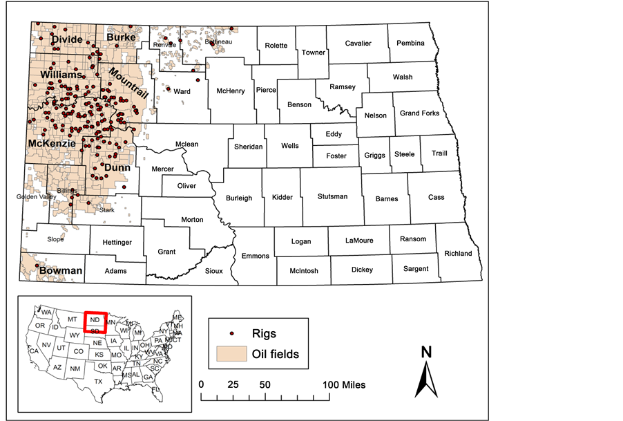
Figure 1. A map reflecting the study location (Note: Rig locations in June 2014 [8] ).

Figure 2. Statewide monthly oil production in North Dakota, separated by major and minor oil producing counties, from December 1953 to January 2014 (NDIC DMR, 2014).

Figure 3. Monthly oil production in North Dakota’s major oil producing counties, separately and in aggregate, from De- cember 2005 to January 2014 (NDIC DMR, 2014).
Varied levels of productivity among these counties within the Bakken Formation is a function of several interacting factors, including location of ground water, extent and depth of oil source rocks, and the number of oil currently developed [21] . In January 2014, the major oil counties produced 82.5% of the statewide production―with Dunn, McKenzie, Mountrail and Williams Counties producing 15.3%, 29.2%, 24.4% and 13.7%, respectively―while the minor counties produced only 7.9% of the statewide total―2.5% in Bowman County, 1.5% in Burke County, and 3.9% in Divide County.
2. Data and Methods
The original data for this research were downloaded from the online databases of North Dakota Drilling and

Figure 4. Monthly oil production in North Dakota’s minor oil producing counties, separately and in aggregate, from De- cember 2005 to January 2014 (NDIC DMR, 2014).
Production Statistics, provided by the Oil and Gas Division of the North Dakota Industrial Commission’s Department of Mineral Resources [8] . Monthly oil production data (in thousand bbl.) were collected from the databases from March 1970 to January 2014, for each of the major and minor oil counties, and for North Dakota as a whole. Table 1 presents summary statistics of monthly extraction for each county, the assorted groups, and North Dakota. The high standard deviations of the major oil production and minor oil production groups during the study period can be attributed to recent, rapid changes in monthly extraction related to the current oil boom.
Stock and Watson [22] explain that trends and breaks make the most important econometric problem in time series―that is, nonstationarity. Due to severe North Dakota winters and recent rapid oil development in most counties, monthly oil production for the state, both production groups, and the individual counties exhibit seasonality. An increasing trend is also evident for statewide production and for the major oil production group, but not for the minor oil production group. We suspected the high probability of breaks in the data because the oil boom began suddenly; hence, we applied the modified Chow-test to check for breaks―the Quandt Likelihood Ratio (QLR) test―and found structural breaks around 2006. This matches our intuition about technological change leading to rapidly increasing oil production since the introduction of horizontal drilling with hydraulic fracturing in the Bakken Formation in 2006. Stock and Watson [22] emphasized that if a regression model ignores breaks, then it can lead to biased and/or imprecise forecasts. Thus, in such cases, model estimation should use only data from the period after the break points.
Additionally, serial correlation was present in the data, so the technique of differencing was applied in the S- ARIMA model. Gujarati and Porter [20] explain that if error terms are not serially correlated, lagged endogenous variables can be treated as exogenous. If needed, we used simple and/or seasonal differencing in our models to eliminate serial correlation of the error terms so that lagged variables could be treated as endogenous.
S-ARIMA models were used to forecast oil production and to investigate whether the oil production trend in North Dakota is consistent across the counties in the assorted groups. According to Pindyck and Rubinfeld [23] and Shumway and Stoffer [24] , the shorthand notation for the model was as follows:
 (1)
(1)
where p is the number of autoregressive terms; d is an integer indicating how many times the series must be differenced to achieve stationarity; q is the number moving average terms; P is the number of seasonal autoregressive terms; D is the number of seasonal differences needed to achieve stationarity; Q is the number of seasonal moving average terms; s denotes the length of the seasonal period (12 months for these data).
The S-ARIMA is a product of the non-seasonal part and the seasonal part, and can eliminate seasonally unst-

Table 1. Descriptive statistics: monthly oil production from January 1970 to January 2014, for each county, for the major and minor groups, and for North Dakota, in millions of barrels.
able effects (i.e. nonstationarity) by using differencing. This model was processed by a few steps in this paper. First, we identified whether the S-ARIMA model is appropriate for the data by analyzing plots of the autocorrelation and partial autocorrelation functions, Akaike Information Criterion, and the QLR test described above. Second, we found the S-ARIMA models with the Least Root Mean Square Error to measure the accuracy for forecasting, and compared estimated coefficients’ p-values with the 10%, 5% and 1% significant levels. Third, we forecasted future oil production with the estimated models.
3. Empirical Results
The statistical results of the QLR tests to check for structural changes in the oil development trend are summarized in Table 2. Each of the individual counties had a break point around September 2006. The break points for North Dakota as a whole and the major oil production counties as a group were also in the year the year 2006, while the break point for the minor oil producing counties as a group was January 2004.
The empirical estimation results of the S-ARIMA models of oil production for each county, for each production group, and for North Dakota as a whole are shown in Tables 3-5. The regression results in the three tables show model type, estimated model parameters, mean absolute error (MAE), R² (goodness of fit), Ljung-Box Chi-Square test for error autocorrelation (lag 2), Augmented Dickey-Fuller (ADF) test for trend, and Seasonal Dickey-Fuller (SDF) test for trend.
The S-ARIMA forecasts results for two production groups and for the state are given in Table 3. The model type and parameters for North Dakota as a whole and for the major oil production group are very similar, and the models are also similar in terms of goodness of fit. This result is not surprising, however, considering that more than 80% of total oil production in the state is attributable to McKenzie, Mountrail, Dunn and Williams counties―the counties in the major production group. All the three groups now have stationary series and no autocorrelations of lags 1 through 2 in the prediction error after being regressed. Given high goodness of fit (R2), oil production in North Dakota will be expected to continue to increase as long as technically recoverable reserves are not exhausted and demand for oil does not decrease.
Table 4 shows forecasting results for each county in the major oil production group. McKenzie, Williams, and Dunn counties are affected primarily by seasonal autoregressive terms, rather than simple lags. All four models have highly statistically significant and positive coefficients, so the future oil production in this group is forecasted to increase. In reality, the oil extraction infrastructure, as well as industrial and commercial districts, in these four counties has been growing rapidly to support the current oil boom. The estimated models for the four individual counties in the major oil production group, which show increasing oil development trends, are consistent with the estimated model for the major oil production group as a whole, as shown in Table 3.
Table 2. Quandt Likelihood Ratio test and break points for each county, major and minor production groups, and North Dakota.
Note: The null hypothesis of QLR Test is no break; the p-values are in parenthesis.
Table 3. S-ARIMA estimation results for the minor and major production groups and for North Dakota.
Note: AR (1) is autoregressive lag 1; AR (2) is autoregressive lag 2; SAR (12) is seasonal autoregressive lag 12; SMA (12) is seasonal moving average lag 12; the standard errors are in parentheses; *, ** and *** indicate significance at 10%, 5% and 1%, respectively; the null hypothesis of Ljung-Box Chi-Square test (lag 2) is that the autocorrelations of lag 1 through 2 in the prediction error are zero; the ADF test and SDF test have the null hypothesis of a unit root, that is, a stochastic trend; “N/A” means that the results are not available.
Table 4. S-ARIMA estimation results for each county in major oil production group.
Note: AR (1) is autoregressive lag 1; AR (2) is autoregressive lag 2; SAR (12) is seasonal autoregressive lag 12; SMA (12) is seasonal moving average lag 12; the standard errors are in parenthesis; *, ** and *** indicate significance at 10%, 5% and 1%, respectively; the null hypothesis of Ljung-Box Chi-Square test (Lag 2) is that the autocorrelations of lag 1 through 2 in the prediction error are zero; the ADF test and SDF test have the null hypothesis of a unit root, that is, a stochastic trend; “N/A” means that the results are not available.
In Table 5, the autoregressive lag coefficients for Bowman County are negative and significant, indicating oil production in this county has been decreasing. Bowman County is the most distant study area in the Bakken Formation, and oil producers are intensively developing oil fields in the four counties which lie at the heart of the Bakken Formation, so production in Bowman County may be expected to decrease in the near future. The oil production of the other two counties―Divide and Burke―has been increasing, and is likely to continue this trend. Burke County shows positive and significant autoregressive and seasonal moving average lag coefficients. Divide County also shows the positive and significant autoregressive and seasonal moving average lag coefficients, which together are much stronger than the negative and significant second autoregressive lag coefficient. Divide and Burke counties, which are near Williams and Mountrail Counties from the major production group, are also experiencing rapid oil development in recent years similar to that of the major group.
The estimated models have been used to forecast oil production in each county (models from Table 4 and Table 5) and North Dakota (model from Table 3) for February 2014 to January 2020. The forecasted monthly production totals from the S-ARIMA models for each county and for North Dakota as a whole are listed in Table 6 from the present through January 2020. The results forecast that oil production in North Dakota would be
Table 5. S-ARIMA estimation results for each county in minor oil production group.
Note: AR (1) is autoregressive lag 1; AR (2) is autoregressive lag 2; SMA (12) is seasonal moving average lag 12; the standard errors are in parenthesis; *, ** and *** indicate significance at 10%, 5% and 1%, respectively; the null hypothesis of Ljung-Box Chi-Square test (lag 2) is that the autocorrelations of lag 1 through 2 in the prediction error are zero; the ADF test and SDF test have the null hypothesis of a unit root, that is, a stochastic trend; “N/A” means that the results are not available.
Table 6. Forecasted monthly oil production for each county and North Dakota from July 2014 to January 2020 in six-month intervals, millions of barrels.
41.18 million bbl. in January 2020, which is a 40% increase relative to January 2014. It also amounts to 19% of current total U.S. crude oil production―222.224 million bbl.―and 1.7% of world oil production―2.29 billion bbl.―in March 2013 [25] . The sum of forecasted production values from the seven major and minor oil production counties of the Bakken Formation in January 2020 is 40.74 million bbl., which accounts for 98.9% of the North Dakota’s total forecast for the same period. The remaining 1.1% would come from other counties in the state. This result is not surprising because the share of North Dakota’s total crude oil production coming from the Bakken has shown an increasing trend since the year 2000. Mason [2] suggests it is technically feasible for the Bakken Formation to produce 1.5 million bbl. per day by 2023. The forecasts presented in our research translate to approximately 1.36 million bbl. per day. Based on these forecasts, the cumulative oil production in North Dakota from January 1970 to January 2020 would be 4.95 billion bbl., which is a small fraction of the estimated 300 billion bbl. of technically recoverable oil reserves reported by Flannery and Kraus [5] .
For each North Dakota county in the Bakken Formation, excluding Bowman County, oil production will continue to increase―especially in McKenzie and Mountrail Counties, where production is predicted to increase sharply. Figure 5 shows historical and forecasted oil production in North Dakota from January 2006 to January 2020, along with upper and lower 95% confidence limits for both the historical period and the forecasting period.
4. Conclusions
The purpose of this paper was to forecast how much oil can be produced in North Dakota for the next five years using the S-ARIMA. Nonstationarity derived from a stochastic trend and the abrupt structural change of oil industry was a big potential problem to our monthly oil production time series. Through the QLR Test, we found break points, which allowed us to select a model fitting period suitable for the S-ARIMA method to provide accurate statistical inference for the historical period, and we hoped good forecasts of future production.
The forecasting results will be useful to the federal government in planning for domestic energy security, and to oil producers and state and local governments in the state of North Dakota as they plan production and infrastructure. The oil production forecasts were produced using separate time series data and models for North Dakota as a whole, for the major and minor oil production groups and for each of the groups’ constituent counties. Excluding Bowman County, the oil development trends for the individual counties of the North Dakota Bakken Formation―i.e. Burke, Divide, Dunn, McKenzie, Mountrail and Williams―and for North Dakota as a whole are consistently increasing and the overall trend is highly likely to continue.

Figure 5. Monthly oil production for North Dakota, from January 2006 to January 2012, and forecasts, from February 2014 to January 2020, with upper and lower 95 % confidence limits.
One caveat is that structural changes in the transportation fuels markets could reduce the accuracy of time series methods for forecasting. For example, if a new technology for oil extraction were developed in the near future that made oil extraction in the Bakken Formation more efficient, this might lead to actual extraction levels during the forecasting period being much higher than our forecasts. On the other hand, if a new liquid transportation fuel became available that could readily replace gasoline at a lower cost, oil extraction in the Bakken Formation and other places would likely diminish. In either of these scenarios, S-ARIMA and other time series models would fail to predict the future accurately.
What we can predict with great certainty, however, is that North Dakota’s influence over domestic and global oil supply systems will increase in the near future, especially over the next five to six years. This is good news for those who are concerned about domestic energy security in the USA.
Acknowledgements
This research was supported by Mountain-Plains Consortium, which is sponsored by the USA Department of Transportation through its university Transportation Centers Program. The contents are sole responsibility of the authors. The authors also would like to thank anonymous reviewers for their constructive comments.
References
- USA Department of Agriculture, National Agricultural Statistics Service (2014) 2009 Agricultural Statistics Annual. http://www.nass.usda.gov/Publications/Ag_Statistics/2009/
- Mason, J. (2014) Bakken’s Maximum Potential Oil Production Rate Explored.
- LeFever, J. and Helms, L. (2006) Bakken Formation Reserve Estimates.
- Williams, J. (1974) Characterization of Oil Types in Williston Basin. American Association of Petroleum Geologists Bulletin, 58, 1243-1252.
- Flannery, J. and Kraus, J. (2006) Integrated Analysis of the Bakken Petroleum System, USA Williston Basin. Search and Discovery Article #10105.
- USA Energy Information Administration (2013) United Arab Emirates. http://www.eia.gov/countries/cab.cfm?fips=TC
- USA Geological Survey (2008) 3 to 4.3 Billion Barrels of Technically Recoverable Oil Assessed in North Dakota and Montana’s Bakken Formation. http://www.usgs.gov/newsroom/article.asp?ID=1911#.UfKlexgo5Lg
- North Dakota Industrial Commission (2014) Review of North Dakota Petroleum Council Flaring Task Force Report and Consideration of Implementation Steps.
- USA Energy Information Administration (2012) North Dakota Oil Production Reaches New High in 2012, Transported by Trucks and Railroads. http://www.eia.gov/todayinenergy/detail.cfm?id=10411
- The White House (2010) Remarks by the President on Energy Security at Andrews Air Force Base. http://www.whitehouse.gov/the-press-office/remarks-president-energy-security-andrews-air-force-base-3312010
- Funke, M. (1992) Time-Series Forecasting of the German Unemployment Rate. Journal of Forecasting, 11, 111-125. http://dx.doi.org/10.1002/for.3980110203
- Ho, S. and Xie, M. (1998) The Use of ARIMA Models for Reliability Forecasting and Analysis. Computers and Industrial Engineering, 35, 213-216. http://dx.doi.org/10.1016/S0360-8352(98)00066-7
- Kelikume, I. and Salami, A. (2014) Time Series Modeling and Forecasting Inflation: Evidence from Nigeria. The International Journal of Business and Finance Research, 8, 41-51.
- Koutroumanidis, T., Iliadis, L. and Sylaios, G.K. (2006) Time-Series Modeling of Fishery Landings Using ARIMA Models and Fuzzy Expected Intervals Software. Environmental Modelling and Software, 21, 1711-1721. http://dx.doi.org/10.1016/j.envsoft.2005.09.001
- Meyler, A., Kenny, G. and Quinn, T. (1998) Forecasting Irish Inflation Using ARIMA Models. Central Bank of Ireland, Dublin.
- Wang, Y.J., Wang, G.Z. and Dong, Y. (2012) Application of Residual Modification Approach in Seasonal ARIMA for Electricity Demand Forecasting: A Case Study of China. Energy Policy, 48, 284-294. http://dx.doi.org/10.1016/j.enpol.2012.05.026
- Ayeni, B. and Pilat, R. (1992) Crude Oil Reserve Estimation: An Application of the Autoregressive Integrated Moving Average (ARIMA) Model. Journal of Petroleum Science and Engineering, 8, 13-28. http://dx.doi.org/10.1016/0920-4105(92)90041-X
- Ediger, V.S., Akar, S.A. and Ugurlu, B. (2006) Forecasting Production of Fossil Fuel Sources in Turkey Using a Comparative Regression and ARIMA Model. Energy Policy, 34, 3836-3846. http://dx.doi.org/10.1016/j.enpol.2005.08.023
- Ediger, V.S. and Akar, S. (2007) ARIMA Forecasting of Primary Energy Demand by Fuel in Turkey. Energy Policy, 35, 1701-1708. http://dx.doi.org/10.1016/j.enpol.2006.05.009
- Gujarati, D. and Porter, D. (2009) Basic Econometrics. McGraw-Hill, New York.
- Kadrmas, Lee & Jackson Inc. (2014) Williston Basin Oil and Gas Related Electrical Load Growth Forecast.
- Stock, J. and Watson, M. (2011) Introduction to Econometrics. Addison-Wesley, Boston.
- Pindyck, R.S. and Rubinfeld, D.L. (1997) Econometric Models and Economic Forecasts. McGraw-Hill, New York.
- Shumway, R.H. and Stoffer, D.S. (2005) Time Series Analysis and Its Applications with R Examples. Springer Science + Business Media, Berlin.
- USA Energy Information Administration (2013) Crude Oil Production. http://www.eia.gov/dnav/pet/pet_crd_crpdn_adc_mbbl_m.htm
NOTES

*Corresponding author.