Natural Resources
Vol.5 No.4(2014), Article ID:44362,16 pages DOI:10.4236/nr.2014.54014
Assessing the Impacts of Summer Range on Bathurst Caribou’s Productivity and Abundance since 1985
Wenjun Chen1*, Lori White1, Jan Z. Adamczewski2, Bruno Croft2, Kerri Garner3, Jody S. Pellissey4, Karin Clark2, Ian Olthof1, Rasim Latifovic1, Greg L. Finstad5
1Canada Centre for Remote Sensing, Natural Resources Canada, Ottawa, Canada
2Environment and Natural Resources, Government of the Northwest Territories, Yellowknife, Canada
3Tlicho Government, Behchoko, Canada
4Wek'èezhìi Renewable Resources Board, Yellowknife, Canada
5School of Natural Resources and Agricultural Sciences, University of Alaska, Fairbanks, USA
Email: *wenjun.chen@NRCan.gc.ca
Copyright © 2014 by author and Scientific Research Publishing Inc.
This work is licensed under the Creative Commons Attribution International License (CC BY).
http://creativecommons.org/licenses/by/4.0/


Received 13 January 2014; revised 17 February 2014; accepted 14 March 2014
ABSTRACT
Barren ground caribou are one of the most important natural resources for northern aboriginal peoples in Canada, and their responsible management has been identified as a top priority by northern communities and governments. This study is aimed to assess the impacts of summer range forage availability and quality on Bathurst caribou’s productivity and abundance. Despite well documented effects of habitat nutrition on individual animal, few studies have been able to link nutrition and population demographics in a quantitative fashion, probably because caribou productivity and abundance could be potentially affected by many factors (e.g., habitat, harvest, predators, diseases/parasites, extreme weather, climate change, industrial development, and pollution), and yet long-term data for many of these factors are not available. By determining the upper envelope curve between summer range indicators and caribou productivity, this study made such assessment possible. Our results indicate that summer range indicators derived from long-term remote sensing time series and climate records can explain 59% of the variation in late-winter calf:cow ratio during 1985 and 2012. As a measure of caribounet productvitiy, the late-winter calf:cow ratio, together with the mortality rate, in turn determined population dynamics.
Keywords:Barren Ground Caribou; Late-Winter Calf:Cow Ratio; Summer Range; Leaf Biomass; Phenology; Remote Sensing

1. Introduction
The Bathurst caribou herd declines 93% from 1986 to 2009 [1] . Similar declines also occurred for many other migratory barren ground caribou herds in northern Canada in the 2000s (http://caff.is/carma). Despite trends towards cash economies (e.g. oil and mineral extraction and tourism), subsistence harvesting of caribou and other wildlife remains a central part of the culture and relationship with the land of aboriginal peoples in Arctic North America [2] . Responsible and sustainable management of caribou to allow for recovery and increased harvesting opportunities has been identified as a priority by many northern communities and governments [3] .
Caribou are affected by many natural and human factors through the year, including habitat, harvest, predators, diseases/parasites, extreme weather, climate change, industrial development, and pollution [2] [4] [5] . While the assessment of cumulative impacts often focuses on manageable human activities [6] , we argue the impact of natural factors could be also critical. Sometimes the effect of human activities could be completely masked by that of natural factors (e.g., implementation of a new harvest regulation during a period of deteriorating habitat conditions). Conclusions drawn by directly linking the harvest regulation with changes in caribou productivity thus could be misleading, without first quantifying and removing the impacts of natural factors. To assess the impacts of these natural factors, long-term data can be very useful because changes in caribou productivity and abundance are usually on the time scale of multi-year to decadal. For some factors, such as diseases and parasites, long-term data sets are scarce. Fortunately, the existence of historical satellite remote sensing records (e.g., NOAA Advanced Very High Resolution Radiometer (AVHRR) since 1980s) makes it possible to develop long-term datasets for caribou habitat indicators that can be assessed against caribou demographic indicators.
In this paper, we will focus on the development of long-term habitat indicators for the summer range of the Bathurst caribou herd, to complement existing studies on the winter range and calving grounds [7] -[9] . We were particularly interested in whether these measures of summer range were related to indicators of caribou productivity and population trend. The key objectives of this study thus are 1) to use historical remote sensing records and field measurements to develop a set of indicators that describe changes in Bathurst summer range forage availability and quality (e.g., leaf biomass, phenology, and nitrogen content); and 2) to assess correlations between these summer range indicators and changes in caribou productivity (e.g., calf:cow ratios, survival rates) and abundance.
2. Materials and Method
2.1. Study Area and Data Sources
The Bathurst summer range study area is located in the northeast portion of Northwest Territories and southwest Nunavut, Canada (Figure 1). Every spring, cows and juveniles from the Bathurst herd migrate from the forested winter ranges in Northwest Territories and northern Saskatchewan to the calving grounds on the tundra in Nunavut. After calving, the cows and calves disperse across their tundra summer range. Ranging from latitude 63˚50' to 66˚27'N and longitude 107˚31' to 114˚43'W, the boundary of the Bathurst caribou summer range was delineated using satellite collared cow location data [9] . In the southwest, it coincides approximately with the dotted black tree line in Figure 1.
A number of studies reported Bathurst caribou calf:cow ratios at peak of calving, fall calf:cow ratios, latewinter calf:cow ratios, calf survival rates, cow survival rates, and population size [1] [10] -[12] . In this study, we used data compiled and updated by Boulanger et al. [1] , Jan Adamczewski and Bruno Croft (personal communication, 2013). In total, there were 10 calf:cow ratios measured at peak of calving, 8 fall calf:cow ratios, 21 late-winter calf:cow ratios, 8 estimates of calf survival rates,13 estimates of cow survival rates, and 6 population change rates established from calving photo surveys between 1985 and 2012. In this study we used the late-winter calf:cow ratio to represent caribou productivity because it has most data points among productivity variables, and is a measure of caribou net productivity. Surveyed usually during March and April for the Bathurst caribou herd [1] [10] , it is directly linked with the birth rate and the calf survival rate in previous year. After calves become yearlings, their survival rate improves substantially.
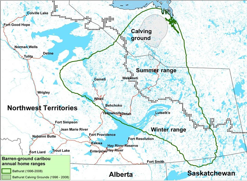
Figure 1. Location of Bathurst caribou summer range between the green boundary line and the dotted black tree line, defined by satellite collared cows GPS data during 1996-2008.
To take advantage of their long historical data records and ongoing capacity, AVHRR data were used in this study for monitoring seasonal and long term changes in leaf biomass and phenology over the Bathurst caribou summer range. The 1-km spatial resolution 10-day composite AVHRR data over the summer range during 1985-2011 were processed with an improved methodology for geo-referencing and compositing, correction for viewing and illumination conditions [13] , cloud screening [14] , and atmospheric correctionby a Canada Centre for Remote Sensing team [15] . The compositing was based on the selection of pixels with the lowest cloudiness index during the compositing interval [14] . The values of the cloudiness index range from 0 (or cloud probability C = 0%) to 255 (or C = 100%). BRDF corrected AVHRR band 1 (surface red reflectance ρr), band 2 (surface near-infrared reflectance ρnir), cloudiness index data, and their actual acquisition date were used in this study. To correct the bias caused by change in AVHRR sensors over the years, Latifovic et al. [16] derived inter-sensor normalization coefficients. We applied these inter-sensor normalization coefficients for AVHRR data used in this study.
As Figure 2 shows, the changes in leaf biomass and phenology were analyzed for each land cover class in the Bathurst caribou summer range, using the circa 2000 Landsat-derived land cover map over the Bathurst summer range developed by Olthof et al. [17] . To match the AVHRR scale, we aggregated the 30-m land cover map into 1-km resolution. Table 1 shows the number of 50% “pure” 1-km land cover pixels (i.e., 50% of the 30-m Landsat-derived land cover classes within a 1-km by 1-km areabelonging to the class) in the Bathurst caribou summer range. In order to apply the unbiased and objective seasonal profile construction method [18] , we combined all shrub dominated classes into one broad shrub class. The same was done for the broad lichen low vegetation class.
To calibrate these AVHRR-derived products, we measured leaf biomass and percentage cover of vascular plants at 27 tundra sites during July 18-27, 2005 around the Lupin Gold Mine, Nunavut, and Yellowknife, NWT. The Lupin Gold Mine is within the Bathurst caribou summer range, while Yellowknife is near its southwest edge. Each site was selected to be relatively homogenous and of a minimum size of 90-m × 90-m [19] [20] . At each site, we sampled five 1-m × 1-m plots (i.e., four plots in four directions at 30 m apart and a random plot). At each plot, percentage covers of vascular plant species were visually recorded in the field and corrected using
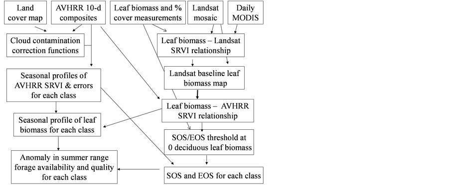
Figure 2. Flow chart showing the steps for monitoring leaf biomass and phenology changes in the Arctic using satellite remote sensing data and field measurements.

Table 1. Number of 50% pure AVHRR pixels in a land cover class in the Bathurst summer range. Also included are % cover of evergreen shrubs and SOS/EOS AVHRR SRVI threshold for the 3 broad land cover classes.
digital photos on a later date [20] . All plants were then harvested, identified to species, sorted into dead and live as well as leaves and stems, and weighted in the field. A sample of these leaves and stems were also taken to the laboratory and oven-dried and weighed to obtain the oven-dry leaf biomass. The values of leaf biomass and percentage cover at each site were calculated as the average of all plots at the site, and sampling errors as the standard deviation divided by the square root of sample size.
To bridge the scale difference between leaf biomass measurement sites and AVHRR pixels, we used the 30-m resolution Landsat images to scale-up the field measurements to 1-km AVHRR resolution. We developed a Landsat mosaic over the Bathurst caribou habitat using 32 cloud-free circa 2000 scenes, following Chen et al. [21] : first selected a cloud-free middle-summer reference scene, and then added other scenes to the reference using overlapping areas’ correlations. Daily 250-m data of the Moderate Resolution Imaging Spectroradiometer (MODIS), which acquires data daily approximately 15 min after Landsat data in the same polar orbit, were used to correct the Landsat-derived vegetation index values to the dates of field measurements.
The climate data used as inputs for simulating the leaf nitrogen content at peak leaf biomass were from the online Canadian Daily Climate Database (http://climate.weatheroffice.gc.ca/climateData/canada_e.html). The Lupin climate station (65˚46'N, 111˚15'W) has the longest records of daily air temperature and precipitation (since January 1, 1982) within the Bathurst summer range and thus were used to represent the summer range.
2.2. Methods for Estimating Leaf Biomass, Phenology, and Leaf Nitrogen Content
In order to use AVHRR time series for monitoring changes in leaf biomass and phenology over the Bathurst caribou summer range, we need to overcome a number of methodological challenges. 1) Construction of seasonal profiles of AVHRR vegetation indices (e.g., simple ratio vegetation index SRVI = ρnir/ρr, the normalized difference vegetation index NDVI = (ρnir − ρr)/(ρnir + ρr)). Although SRVI, NDVI, and many other satellite remote sensing-derived vegetation indices can be used for monitoring leaf biomass and phenology [21] [22] , the SRVI was found to be the best linear fit to leaf biomass at sites across the Canadian Arctic [21] and therefore is used in this study. AVHRR-derived vegetation indices usually have a high noise to signal ratio caused by residue cloud contamination and aerosol variations. Despite substantial pre-processing efforts, the residue cloud contamination could still cause significant bias in AVHRR SRVI [23] . In addition, the variation in aerosols could result in up to ~40% random error in AVHRR SRVI for a clear sky single pixel [21] . 2) Calibration of remotely sensed leaf biomass estimates using field measurements due to tempo-spatial mismatches between AVHRR SRVI and field measurements. Because it was difficult to find sites several km across, field leaf biomass measurement sites were chosen to be at least 90 m by 90 m, in contrast to the 1-km AVHRR spatial resolution. Additionally the field measurements were conducted during mid-summer in 2005, whereas AVHRR SRVI values were over the entire growing season every year from 1985 to 2011. 3) Definition of AVHRR SVRI threshold for the start and the end of growing season (SOS and EOS, respectively). Nearly all current satellite phenology monitoring methods define SOS/EOS in some arbitrary way, which makes the resultant phenology dates methodologically dependent and thus less credible [24] .
To address the 1st challenge, we divided AVHRR pixels in a given composite period for a land cover class into 4 categories: clear sky (C = 0% - 20%), lightly (C = 20% - 40%), moderately (C = 40% - 60%), and heavily cloud contaminated (C > 60%) [18] . The underestimation of AVHRR SRVI over cloud contaminated pixels was corrected using the bias coefficients in Table 2. The corrected AVHRR SRVI values over cloud contaminated pixels as well as that over clear sky pixels of the land cover class for the given composite period were weighted using their area fractions to arrive at their final corrected value of AVHRR SRVI, from which the seasonal profiles of AVHRR SRVI for the class were thus objectively constructed. The corresponding uncertainties in AVHRR SRVI are composed of random errors over clear sky pixels and uncertainties of cloud contaminated pixels [25] .
The 2nd challenge was resolved using an up-scaling outlined in Figure 2. 1) We developed relationship between Landsat SRVI and field leaf biomass measurements. Because the date of Landsat SRVI was different from the date of field measurements, MODIS data on both dates were used to correct the Landsat-derived vegetation index values to the middle date of field measurements, via the relationships for ρr and ρnir between Landsat and MODIS. 2) Applying the relationship between Landsat SRVI and leaf biomass to the Landsat mosaic, we produced a baseline map of leaf biomass for the Bathurst summer range (Figure 3). 3) We developed the relationship between clear-sky AVHRR SRVI (RsA) and corresponding 1-km resolution leaf biomass (Bl, in g∙m−2) aggregated from the leaf biomass baseline map:
 (1)
(1)
The standard estimate error of Equation (1) is 10.8 g·m−2, R2 = 0.68, p-value = 2.5 × 10−205, and n = 833. To reduce the random error in AVHRR SRVI for a clear sky pixel, we averaged RsA and Bl to a window of 25 pixels, as a compromise between final accuracy in the averaged RsA and a large enough sample number for the regression [21] . The robust (TheilSen) regression was also used for driving Equation (1) to avoid the impact of outliers [26] . 4) Applying Equation (1) to the seasonal profiles of AVHRR SRVI, we calculated the seasonal and long term changes in leaf biomass.
For the 3rd challenge, we defined SOS (or EOS) in a biophysically meaningful and objective manner, namely, as the day of year on which the biomass of green leaves of the deciduous shrubs and herbs equaled 0 in the spring (or fall). Due to the existence of evergreen shrubs in most tundra sites, the SOS/EOS AVHRR SRVI threshold ( , where superscript T stands for threshold) should thus be determined by considering contributions
Table 2. Statistics for linear regressions between  and
and  (or
(or ,
, ). The bias shows correction needed from
  (or
(or ,
, ) to
) to , SEE is the standard error divided by ensemble mean
 , and N is the number of qualified composite periods. We calculated the ensemble mean
  by averaging over all qualified composite periods.
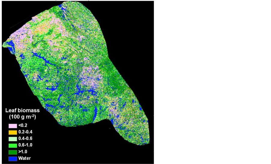
Figure 3. Landsat-derived circa 2000 leaf biomass map over the Bathurst caribou summer range.
from both deciduous and evergreen components. By definition,  . In turn
  where
where  and
and  are, respectively,
  of evergreen shrubs and that of other components, and Pes is the percentage cover of evergreen shrubs. Similarly,
  , where
  and
and  are, respectively,
  of evergreen shrubs and that of other components. Replacing
  (or
(or ) with
  (or
(or ), the AVHRR SRVI of evergreen shrubs (or other components) on the day of SOS/EOS, we have
 (2)
(2)
The value of  can be obtained by inverting Equation (1) and setting Bl = 0, because the leaf biomass-SRVI relationships in the Arctic are usually dominated by deciduous plants that are taller and have higher SRVI value. The values of Pes for different land cover classes in the Bathurst caribou summer range were estimated using field measurements (Table 3). We determined the value of
 , on the basis of the reported values of 0.04 for heather and 0.04 for crowberry [27] . Similarly,
  , averaged from reported values of 0.06 for mosses, 0.17 for lichen, 0.07 for peats, 0.08 for dead grass, and 0.08 for wet soil [27] -[29] . The measurements by Peltoniemi et al. [27] also gave a mean value of in-situ NDVI of evergreen shrubs to be 0.68, averaged from its values of 0.66 for heather and 0.70 for crowberry. However, this in-situ NDVI cannot be directly used for determining
  for the following two reasons: the near infrared band of AVHRR includes the major part of the red edge area around 700 nm, and covers the strong water vapor absorption area from 900 - 1000 nm, both of which could substantially reduce the ρnir value in comparison with in-situ measurements [30] . On the basis of two years measurements at grass savannah sites in Senegal, Africa in 2001 and 2002, Fensholt and Sandholt [30] reported two relationships between in situ NDVI measurements and those derived from AVHRR, with R2 ranging from 0.64 to 0.75. In this study, we took their average, given by:
 (3)
(3)
Inserting the in-situ evergreen shrubs’ NDVI value of 0.68 into Equation (3), we have an AVHRR equivalent evergreen shrubs’ NDVI = 0.25. From the relationship between NDVI and SRVI (i.e., SRVI = (NDVI+1)/(1−NDVI)), we have . The final values of SOS/EOS AVHRR SRVI threshold for each class were listed in Table 3.
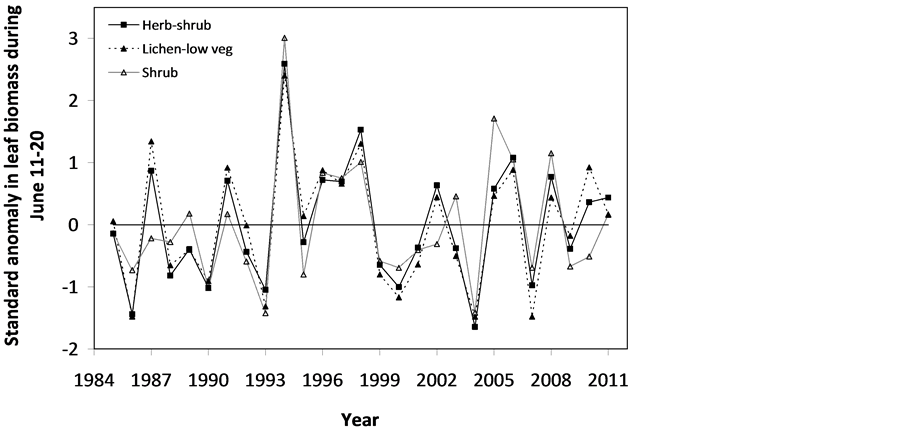
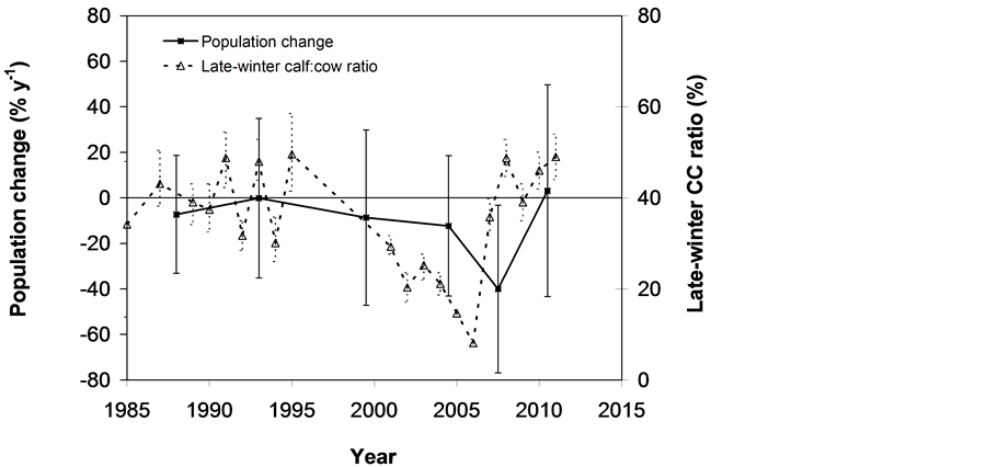
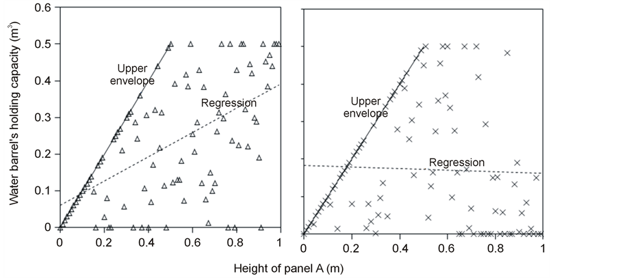
The SOS date was then determined as the day of year at which AVHRR SRVI became>the threshold in the spring for each land cover class in the summer range. Similarly, the EOS date was determined as the day of year at which AVHRR SRVI became Even small variations in forage quality in the summer range can strongly influence caribou body growth and development through a multiplier effect [31] . Leaf N concentration and forage digestibility are two commonly used measures of forage quality [32] [33] . Without adequate measures of forage digestibility and because forage digestibility is positively correlated with leaf N concentration when the latter is <3% [32] [33] , we used only leaf N concentration in defining the forage quality measure in the summer range. Measurements on reindeer ranges of the Seward Peninsula in Alaska show seasonal patterns in leaf N concentration [32] : peaking at or near the beginning of the growing season with leaf N concentrations between 2% - 6%, decreasing rapidly and then stabilizing around 1% - 3% toward the middle of the growing season, and decreasing further near the end of growing season. The review by Johnstone et al. [34] showed a similar pattern of N concentration in key caribou forage groups across North America, except evergreen shrubs that showed no clear seasonal pattern. The decrease in leaf N concentration from the beginning to the middle of growing season was the result of N dilution caused by the increase in foliage biomass significantly exceeding the supply from root N uptake and transfer of Nresorbed in the previous year from storage organs to leaves. The decrease in leaf N concentration near the end of growing season was likely due to N resorption before senescence [35] . Because the leaf N concentration at peak leaf biomass is relatively stable and positively correlated with leaf N concentration at senescence, we selected it as the forage quality measure for the summer range. We quantified the forage quality measure using the remotely sensed leaf biomass and the N allocated to foliage biomass estimated using a fully coupled carbon-nitrogen cycle model [36] . The model was calibrated with two growing seasons’ leaf N concentration measurements on reindeer ranges of the Seward Peninsula [32] , and those during 2004-2008 over Canada’s Arctic tundra ecosystems (unpublished data). Table 3. AVHRR SRVI threshold of SOS and EOS for different land cover classes in the Bathurst caribou summer range and associated parameters. 2.3. Method for Calculating Caribou Summer Range Indicators Inadequate leaf biomass, late start date and early end date of growing season, and poor quality of leaf biomass are negative for summer range forage availability and quality, and thus might be detrimental to caribou calf growth and the cow regaining body reserves required to become pregnant in the fall. Based on its seasonal pattern, we divided the leaf biomass variable into 5 measures: Bl(1), Bl(2), Bl(3), Bl(4), and Bl(5), respectively, stand for leaf biomass immediately post peak calving from June 11-20, early summer from June 21-July 10, midsummer from July 11-August 10 during which leaf biomass usually peaks and is relatively stable, late summer from August 11-September 20, and late summer-fall from September 21-October 10 (i.e., the last period green leaves might be available). The SOS and EOS are related to Bl(1) and Bl(2), although sometimes the opposite might occur e.g., a late yet rapid green-up can have a high Bl(1) but late SOS. Therefore, SOS and EOS were used as additional forage availability measures. Finally, the leaf nitrogen content at the peak leaf biomass Npb was used to measure the summer range forage quality. To better enable integration and comparison, standardized anomalies have been often used as ecological indicators [37] . The value of the standard anomaly for Bl(1) in year i over land class k was calculated as [25] : where To represent the whole summer range, summer range measure for leaf biomass anomaly from June 11-20 in year i where fa(k) is the area fraction of land cover class k (= 1, 2, and 3 standing for lichen low vegetation, herb shrub, and shrub, respectively). Again the values of the summer range measures for other 7 measures (i.e., SRMlb2, SRMlb3, SRMlb4, SRMlb5, SRMSOS, SRMEOS, and SRMlnc, respectively, for leaf biomass anomalies during June 21-July 10, July 11-August 10, August 11-September 20, September 21-October 10, SOS, EOS and leaf nitrogen content at the peak leaf biomass) can be calculated in the same manner. To investigate the cumulative impact of various combinations of these summer range measures, we constructed summer range cumulative indicators (SRCI). For example, the SRCI5m combines 5 summer range measures as follows: Note that a positive anomaly for EOS has likely negative impact, and so was calculated as minus instead of plus, to ensure a negative SRCI value indicates poor overall forage availability and quality. Other SRCIs were also computed and investigated. 2.4. Method for Assessing Impacts of Summer Range Conditions on Caribou Productivity Because caribou productivity are affected by many factors in a complex manner over time and space, long-term data for all these factors would be preferred to assess their cumulative impacts. However, long term datasets are not available for many factors (e.g., parasites and diseases). Under this circumstance, we were challenged with assessing potential effects of summer range variables on caribou productivity in a timely manner. In order to find an approach that can overcome the challenge, we examined a simple case between the water holding capacity of a water barrel and the height of side panel A. The cubic shaped water barrel has a bottom of 1 m2 and 4 side panels that are 1 m in width and variable in heights, so that its water holding capacity is calculated by the bottom area × the height of the shortest panel. Assuming in one experimental run, we have 100 measured heights of panel A, incrementing evenly from 0 to 0.99 m. The heights of other two panels vary randomly between 0 and 1 m, while the height of panel #4 is a variable representing a rare occurrence event, with 90% of chances having a normal value of 0.5 m and 10% of changes dropping to 0 m. Figure 4 shows the result of two separately experimental runs, from which we can draw the following conclusions. 1) Data points on the upper envelope line represent the cases in which the water barrel’s holding capacity is solely controlled by the Figure 4. A case study for illustrating the usage of upper envelope. (a) (left-hand plate) and (b) (righthand plate) present the results of two separate experimental runs. height of panel A. For points below the upper envelope line, the height of panel A is not shortest and therefore is not a limiting factor. 2) There is an impact saturation point for the height of panel A at 0.5 m. When the height of panel A is taller than its saturation point, the water barrel’s holding capacity is completely determined by the heights of other panels. Therefore, the upper envelope impact line can only be determined for cases when the height of penal A is shorter than the impact saturation point. 3) The slope, intercept, and correlation coefficient R of the linear regression lines vary from one experimental run to another: 0.33, 0.06, and 0.58 respectively for the experimental run in Figure 4(a); and −0.02, 0.18, and −0.04 respectively for that in Figure 4(b). It is also true for all other experimental runs (not shown), although with different statistics. On the other hand, the upper envelope line remains the same for all these experimental runs because it represents the true causal relationship between the height of panel A and the water barrel’s holding capacity. The upper envelope approach applies the principle of limiting factors [38] , which suggests that, at any given time in a particular ecosystem, productivity is constrained by a single, metabolically essential factor that is present in least supply relative to the potential biological demand. It has been used in studies of nature, such as the light response curves between photosynthesis rates and solar irradiance, or the relationships between the marine phytoplankton maximum growth rates and temperature [39] -[41] . The light response curves may be determined in two different ways: 1) using the commonly used least-squares regression if they are measured while all other conditions are optimal; or 2) the upper envelope approach if the measurements are conducted under natural conditions in which water stress, insects damage to leaves, or low (or high) temperature limitation may occur [39] [40] . The upper envelopes may take on different shapes: linear in the case of water barrel’s holding capacity, exponential for the relationships between the marine phytoplankton maximum growth rates and temperature, or the Mitscherlich model for light response curves between photosynthesis rates and solar irradiance. Examining the relationships between caribou productivity (Pc) and a summer range cumulative indicator (SRCI), we found that they are quite similar to the light response curves when measurements are conducted under natural conditions: both are affected by many other unknown factors. Therefore, the Mitscherlich model was used in this study to approximate the upper envelope impact curves of SRCI on caribou productivity: where Pc,max represents the maximum possible value of caribou productivity, S corresponds to the initial slope of the curve at poor summer range conditions, INT denotes the x-intercept, when caribou productivity reaches zero. Similar to the light saturation point of plant photosynthesis, there is also an impact saturation point for a SRCI, which were determined visually in this study. When the values of a SRCI were >the impact saturation point, they were excluded from the determination of the upper envelope curves. 3. Results 3.1. Changes in Summer Range Forage Availability and Quality during 1985-2011 Figure 5 shows the standard anomalies of the three broad land cover classes in the Bathurst caribou summer range during June 11-20 from 1985 to 2011. Although the absolute leaf biomass of the shrub class (or the herb-shrub class) was higher than that of the lichen low vegetation class, their standard anomalies were similar. No statistically significant trends were found, except large inter-annual variations. Using Equation (5), we computed the eight summer range measures during 1985 and 2011. Summer range cumulative indicators were then calculated by combining these measures differently. As Figure 6 shows, SRCI5m was the lowest in 2004, followed by that in 2000 and 1988. In 2004, a very late SOS, very early EOS, extremely low leaf biomass during the entire growing season except mid-summer (July 11-August 10) resulted in the lowest SRCI5m. Similar causes were found for 2000 and 1988. Figure 5. Standard anomalies in leaf biomass of the three broad classes of land cover in the Bathurst caribou summer range from June 11-20 during 1985 and 2011. Figure 6. Correspondence between Bathurst caribou late-winter calf:cow ratio and SRCI5m during 1985-2012. 3.2. Correspondence between Caribou Variables and Summer Range Indicators The late-winter calf:cow ratio increased from 35% (i.e., 35 calves:100 cows, and is presented here as 35%) in 1985 to upwards of 40% in the 1990’s, declined sharply to only 8% in 2006, recovered to upwards of 40% during 2007-2011, and a recent drop to 25% in 2012 (Figure 6). The late-winter calf:cow ratio in 1988 appeared to be an outlier and thus was excluded in further analysis (see rationale in Section 4.2). From Figure 6, we found that caribou productivity appears to correspond well with SRCI5m. The value of SRCI5m was about −0.8 in 1988, increased to >−0.3 in 1990’s, declined to −1.07 in 2004, and then recovered to mostly >0. It appeared that the late-winter calf:cow trend lagged the SRCI5m at about 2 years. This agrees well with the fact that biologically the late-winter calf:cow ratio in year i = (the calf:cow ratio at peak calving in year i-1) × (the calf survival rate from peak calving in early June in year i-1 to late-winter in year i)/(the cow survival ratio during the same period). These calf and cow survival rates from peak calving to late-winter in March-April were probably influenced by the summer range conditions in year i-1, while the calf:cow ratio at peak calving in year i-1 was likely affected by the cow pregnancy rate and summer range conditions in year i-2. The changes in the late-winter calf:cow ratio in turn appear to have played a dominant role in population abundance change (Figure 7). The population modeling for the Bathurst herd by Boulanger et al. [1] showed that the level of recruitment needed for stability depends on the adult caribou mortality rate. From Figure 7, it appears that 40% was the approximate equilibrium point between the adult caribou mortality rate and the late-winter calf:cow ratio. For example, the mean late-winter calf:cow ratios were 38%, 41%, 29%, and 46%, respectively, from 1985-1990, 1989-1996, 1995-2009, and 2008-2011. Correspondingly, the rates of caribou population change were −7% per year from 472,000 ± 72,900 in 1986 to 352,000 ± 77,800 in 1990, 0% per year from 352,000 ± 77,800 in 1990 to 349,000 ± 94,900 in 1996, −13% per year from 349,000 ± 94,900 in 1996 to 31,900 ± 11,000 in 2009, and 3% per year from 31,900 ± 11,000 in 2009to 35,000 ± 11,000 in 2012. Unfortunately, there were not sufficient data to quantify the adult caribou mortality rate for the Bathurst herd during these corresponding time periods, which would require mortality rates of cows and bull as well as their sex ratio. Cow mortality rate was available only after 1996, ranging from 4% to 54% [1] , whereas the bull: cow ratios were surveyed only after 2000, ranging from 31% to 63% [10] [11] . Bull mortality rate was suggested to be higher than females especially if environmental conditions were poor, but there was no actual data. These numbers suggest that 40% adult caribou mortality was possible, although with a high variability. The variability might be further increased by the effect of harvest. For example, the importance of harvest increased as abundance became low from 1996-2009, and could further accelerate the population decline. On the other hand, the major harvest reduction implemented since 2009 might have contributed to its population stabilization. Figure 7. Correspondence between Bathurst caribou late-winter calf:cow ratio and rate of caribou population change from 1985-2012. 3.3. Impacts of Summer Range Change on Caribou Productivity Individual SRM, as well as their various combinations in the form of SRCI were investigated against the late-winter calf:cow ratios. Since both summer range conditions in year i-1 and i-2 could have influenced the late-winter calf:cow ratio in year i, and it is difficult to attribute their relative importance, we used the minimum value of the two years. These test results indicate that SRCI5mwas the best indicator for the late-winter calf:cow ratio of the Bathurst caribou herd. As Figure 8 shows, the late-winter calf:cow ratio could reach 50% when conditions were favorable, and decrease to 10% when MIN(SRCI5m(i-1), SRCI5m(i-2)) approaching to −1. Values of the late-winter calf:cow ratio below the upper envelope curve as well as in the not limiting zone indicate likely influences of other factors. The fitted Mitcherlich curve (i.e., Pc,max = 51.8%, S =4, and INT = −1.151 in Equation (7)) explained 59% of the variation in late-winter calf:cow ratios during 1985-2012, with R2 = 0.591, P-value = 1.94 × 10⁻⁴, and sample size = 18. The impact saturation point of MIN (SRCI5m(i-1), SRCI5m(i-2)) on late-winter calf:cow ratio was visually determined to be −0.2. For comparison we also fitted a linear regression line through the same 18 data points in the limiting zone, with R2 = 0.54, and P-value = 5.03 × 10⁻⁴. Both relationships are statistically significant at the 99% confidence level. However, the linear regression, which estimates the mean rate of impact by MIN (SRCI5m(i-1), SRCI5m(i-2)) that concurred with actual conditions of other factors, could easily be influenced by other factors through their effects on late-winter calf:cow ratios below the upper envelope curve. The upper envelope curve, on the other hand, was not affected by these other factors and represents the causal relationship in which summer range forage conditions in years i-1 and i-2 were probably the dominant factors limiting the late-winter calf:cow ratio in year i. 4. Discussion 4.1. Advantages and Limitations of Using the Upper Envelope Approach In comparison with the commonly used least-square regression, the upper envelope approach is advantageous because it enables us to approximate the causal relationship in which summer range conditions were likely dominant factors limiting caribou productivity, despite of lacking data from all other factors. Figure 8. Impact of previous two years’ summer range conditions on the Bathurst caribou late-winter calf:cow ratio during 1985 and 2012. Error bar shows one standard error in the late-winter calf:cow ratio. The solid line is the upper envelope impact curve, while the dash line shows their linear regression. Date points in the not-limiting zone were excluded from the derivation of the two lines. On the other hand, the upper envelope approach requires a large enough sample size, which becomes even more difficult to obtain when data points in the not-limiting zone were excluded because they exerted no impact on the upper envelope curve. The same can be said for the data points below the upper envelope curve as they were limited by factors other than the summer range conditions. Out of the 20 data points between the MIN (SRCI5m(i-2), SRCI5m(i-1)) and the late-winter calf:cow ratio in year i, only 7 are right on the curve. Therefore, applications of the upper envelope approach can be difficult for other Bathurst caribou demographic variables (e.g., calf:cow ratio at peak calving, fall calf:cow ratio, survival rates of calves or cows) that have much less available data points. In order to more convincingly determine the upper envelope curves between summer range indicators and caribou productivity variables other than the late-winter calf:cow ratio, continuation of monitoring of both summer range indicators and these caribou productivity variables is essential. Alternatively, it may also be possible to pool together data from different caribou herds, as Bissinger et al. [41] did for the relationships between the marine phytoplankton maximum growth rates and temperature. 4.2. Exclusion of the Calf:Cow Ratio in 1988 as an Outlier We excluded the very high 1988 late-winter calf:cow ratio of 74% as this value seems biologically unrealistic and the field sampling may not have been fully representative of the herd. Survival rates of caribou calves are generally substantially lower than in adults, and low calf:cow ratios are indicative of decline [5] . The Bathurst herd was declining from 1986 to 1990, and the average calf:cow ratios over this period were 38:100, consistent with a slow decline. Assuming a fecundity of 0.82, calf survival in 1988 would have had to be 67%, which seems unlikely for this herd when it was declining after peak abundance. In addition, experience in the field shows that calf:cow ratios can vary spatially, and a misleadingly high calf:cow ratio could result if field sampling was not fully representative of the herd’s distribution. The overall evidence suggests that the 1988 late-winter calf:cow ratio was an outlier and likely was not a true measure of recruitment in that year. Similarly, Boulanger et al. [1] estimated the late-winter calf:cow ratio in 1988 to be 0.38, using ademographic model that simultaneously optimizes all demographic variables. 4.3. Implication of Summer Range Monitoring to Caribou Management Management decisions about harvest that affect hunters and communities are generally made based on caribou population size and trend and the scale of recent harvest. It is important to bear in mind that many other factors will continue to affect caribou productivity and population trend e.g., summer range quality, winter snow conditions, and disease, and it is not just human activities that affect caribou numbers. Despite well documented effects of habitat nutrition on individual animal performance and nutritional strategies of caribou and reindeer [42] -[45] , few studies have been able to link nutrition and population demographics in a quantitative fashion. By determining the upper envelope curve between summer range indicator and caribou productivity, we suggest that an assessment can be made of when the summer range conditions could become limiting. Since changes in summer range conditions precede late-winter calf:cow ratio by 2 years and even longer for that of caribou abundance, timely annual monitoring of these variables could help us to anticipate likely population trend in the herd. Wildlife managers may be able to better attribute cumulative impacts to natural environmental changes and human activities, and thus improve their ability to manage people’s expectations of the herd’s likely short-term trend. 5. Conclusions On the basis of historical AVHRR time series and field measurements of leaf biomass and percentage cover, we developed eight summer range forage availability and quality measures for the Bathurst caribou herd during 1985 and 2011. Among individual summer range measures and their various combinations, SRCI5m was found to be the best summer range cumulative indicator for caribou productivity. Our results indicated good correspondence between SRCI5m and the late-winter calf:cow ratio, with the later lagging the former by two years. The upper envelope curve of MIN (SRCI5m(i-1), SRCI5m(i-2)) explained 59% of the variation in late-winter calf:cow ratio during 1985 and 2012. The late-winter calf:cow ratio, in turn, was strongly related to caribou population trends between 1986 and 2012. Given that summer range conditions have likely been the dominant factors limiting Bathurst caribou productivity in 7 out of 20 years during 1987 and 2012, their monitoring should be continued on a regular basis in order to better inform decision makings on caribou management and industrial developments. Last but not the least, other factors might have also played important roles, or could become important in the future (e.g., an outburst of parasites or diseases or an extreme weather event). Monitoring of these other factors should be initiated or strengthened. Acknowledgements The authors greatly appreciate the financial support from the Northwest Territories Cumulative Impact Monitoring Program (NWT CIMP), and the Remote Sensing Science Program of ESS-NRCan. The guidance, suggestions, and technical assistances from Environment and Natural Resources of GNWT, Tlicho Government, Wek'èezhìi Renewable Resources Board are much appreciated. Drs. Don Russell, Anne Gunn, and Bob White of CARMA network as well as two anonymous reviewers reviewed and provided constructive comments on earlier drafts of the manuscript. References NOTES *Corresponding author. (4)
(4) and
and  are the long-term mean and standard deviation of Bl(1) from 1985-2011. The values of the standard anomaly for other 7 measures can be calculated in the same manner.
 was area weighted:
 (5)
(5) (6)
(6) (a) (b)
 (7)
(7)