Natural Resources
Vol.4 No.1(2013), Article ID:29159,11 pages DOI:10.4236/nr.2013.41003
Bed Forms and Sediment Characteristics along the Thalweg on the Tanana River near Nenana, Alaska, USA
![]()
Civil and Environmental Engineering Department, University of Alaska Fairbanks, Fairbanks, USA.
Email: hatoniolo@alaska.edu
Received October 17th, 2012; revised November 23rd, 2012; accepted December 13th, 2012
Keywords: Sand-Gravel Riverbeds; Dunes; Steepness; Thalweg; Suspended-Sediment Load; Bed Load
ABSTRACT
Sediment sampling and longitudinal river-bottom surveys were conducted along the thalweg on the Tanana River near the city of Nenana, Alaska, USA, to provide basic information for the engineering design requirements of hydrokinetic devices to be deployed in the area. The study reach was located at approximately 64˚33'50"N and 149˚04'W. The Tanana is a large glacier-fed river, with open-water flow conditions from May to October. The river presents a single channel in the study area. Granulometric analyses of sediment moving near the riverbed reveals the coexistence of three distinctive types of sediment along the study reach: 1) nearly uniform fine sand; 2) bimodal distributions containing fine sand and medium gravel; and 3) medium gravel. Preliminary relationships between sediment loads and discharge were developed. Dunes with small superimposed dunes were found along the reach. The basic geometric parameters (i.e., wavelength and height) of dunes were measured, and steepness was calculated. In general, dune wavelength increased with increasing discharge. Dune wavelengths ranged from 41 to 67 m, while small-dune wavelengths ranged from 13 to 16 m. Steepness increased slightly with increasing discharge.
1. Introduction
For decades, river mechanics have received the attention of numerous researchers. Studies have involved field, laboratory, and theoretical work, or combinations thereof. Aspects covered in the literature range from basic hydraulics to fish habitat conditions. An excellent summary of the state of the art in river studies is provided in the recently published ASCE Manual 110 [1].
Generally, a particular set of equations is used for estimating the geometric parameters, roughness coefficient, and sediment transport of sand-bed rivers and gravel-bed rivers. Literature on the different processes of sand-bed rivers is extensive [2-5]. Empirical and mechanistic analyses of gravel-bed rivers are widely available [6-8].
Extensive research has been conducted on dunes as a particular type of bed form. Fernandez et al. [9] reported that dunes are found on sand-bed and gravel-bed rivers. Best [10] completed a comprehensive review of dunes. Numerical work on dune evolution and dune migration is also available [11-13]. Linking dunes and eco-hydrology, Amsler et al. [14] discussed the influence of dunes on macro-invertebrates on the Parana River (Argentina).
Batalla and Martin-Vide [15] studied the coexistence of sand and gravel sediment in rivers. Kleinhans [16] discussed the importance of dunes in sand-gravel river transport processes. Other authors [17-19] presented sediment-transport equations for sand-gravel rivers.
Several publications are available on the variability of bed load [20-24]. Similarly, the literature is vast on samplers, such as the Helley-Smith sampler [25], and/or instruments, such as piezoelectric sensors and geophones, used in the field to calculate bed load [26-29]. The crosssectional variation in suspended sediment load is relatively small compared with the variation in bed load. Several approaches are available for estimating the suspended sediment load. These methodologies consider measurements in a single vertical or in multiple verticals across the entire river width [30]. Thus, the error increases with decreasing number of verticals in the river cross section.
Engineering work conducted in a river setting requires knowledge of local sediment transport conditions and bed form characteristics. With this in mind, basic sediment and bedform data along the thalweg on the Tanana River near the city of Nenana, Alaska, are presented here. The information provided in this article is key to the design of anchoring systems and studies related to blade abrasion of hydrokinetic devices. The characterization of this river reach is part of the ongoing research focused on hydrokinetic resource assessment [31].
2. Study Site
Fieldwork was carried out on the Tanana River near Nenana, Alaska, USA. The approximate midpoint of the study reach is located at 64˚33'50"N and 149˚04'W. The river presents a single channel in the study area, with a relatively straight reach that encompasses the upstream and middle zones, followed by a sharp bend in the downstream area (Figure 1). The riverbank along the reach is formed by relatively fine and cohesive sediment. The outer bank along the river bend is formed by hard rocks, naturally available in that area.
The Tanana River, a tributary of the Yukon River, is a large glacier-fed river that drains approximately 113,959 km2. Glacier-fed rivers are characterized by high sediment loads. The annual suspended-sediment load for the Tanana River at Nenana is estimated at 38 × 106 tons [32].
The United States Geological Survey (USGS) operates a gauging station (ID 15515500) near the study site. Historical average monthly discharge during the open-water season (i.e., May to October) ranges from 495.5 m3/s to 1704.7 m3/s. Figure 2 shows the seasonal hydrograph for year 2010. Winter discharge ranges from 184.6 m3/s to 269.9 m3/s.
3. Equipment
River bottom surveys (and velocity measurements) were carried out using a Teledyne RDI Rio Grande 1200 KHz Acoustic Doppler Current Profiler (ADCP). The ADCP unit was mounted onto a 6-meter-long aluminum boat equipped with a 30 HP outboard motor. A sounding reel (type B-56, Model 3260) and a retractable boom were located at the bow of the boat for sediment sampling. The boat was also equipped with a radio and a NovAtel GPS rover station. A second NovAtel GPS was used as an onshore base station. This GPS system provided realtime kinematic (RTK) positioning to the ADCP.
Suspended-sediment samples were taken with a depthintegrating suspended-sediment sampler type US D-77. Sediment to estimate bed load was captured with a Helley-Smith sampler, Model 8055. These two samplers proved adequate for sampling the Tanana River during the summer months. Smaller and lighter samplers such as a depth-integrating hand-line type US DH-59 and a handheld bed load sampler type US BLH-84 were used in winter (i.e., when the river was ice-covered).
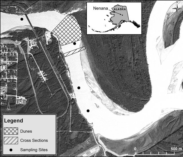
Figure 1. Study site on the Tanana River near Nenana, Alaska, USA. Locations indicated in the figure are approximated.
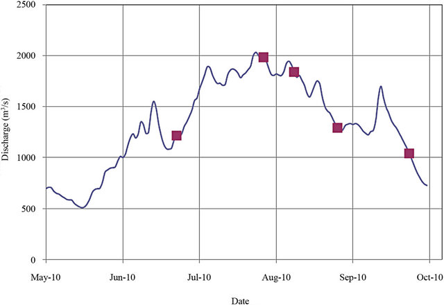
Figure 2. Tanana River, 2010 summer hydrograph. USGS data, station 15515500. Squares indicate fieldwork days.
4. Methodology
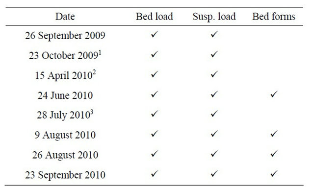
As mentioned before, this work is part of a broader research effort that is focused on hydrokinetic resource assessment. As such, and because of budget and logistical constraints, sediment sampling was done along the thalweg, where kinetic energy is strongest, and thus where deployment of hydrokinetic devices is expected. Initial fieldwork started in September 2009 and consisted only of sediment sampling on a nearly monthly basis during the open-water season. Hence, two field campaigns were carried out in 2009 (in September and October). Suspended sediments were sampled using the US D-77 at different points near the upstream, middle, and downstream portions of the study reach. The Helley-Smith sampler was used to capture sediment moving over the riverbed. Sampling time, based on field conditions, ranged from 2 to 5 minutes. While a limited number of bed load samples were taken during each field visit, it is argued here that the available samples could capture the variability of riverbed sediment load along the thalweg.
Minimal sampling was done during the winter months. In fact, a field crew gathered sediment data in ice-covered conditions on 15 April 2010. The smaller sediment samplers (US DH-59 and US BLH-84) were deployed through holes drilled in the ice. Sampling was done in a couple of holes along a river transect in the study area.
The ADCP was used during the 2010 field season. The first open-water campaign was carried out on 24 June 2010. On that day, dunes were found in the center of the river, immediately upstream of the river bend. This sector was surveyed in subsequent field visits. Sediment sampling was also done. Additional field campaigns were performed on 28 July, 9 August, 26 August, and 23 September. Table 1 provides a summary of dates and the types of data collected each day.
On 9 August 2010, water-surface elevations along the river reach were surveyed by personnel from TerraSond, a hydrographic survey company. These elevations were used to calculate the water-surface slope for that day.
Suspended-sediment concentrations, C, were calculated following the ASTM standard D 3977-97, Method B [33]. Analyses were not performed to establish the sediment grain-size distributions of suspended sediment. However, sieving analyses following the ASTM standard C136-06 [34] were conducted to establish the grain-size distributions of sediment captured by the Helley-Smith sampler. The analyses were conducted at the University of Alaska Fairbanks, Water and Environmental Research Center.
Finally, bed and suspended loads were calculated. It should be noted here that the term suspended load refers to bed material in suspension and wash load. The basic geometric dimensions (i.e., wavelength, λ, and height, Δ) of the dunes were measured, and the steepness, Δ/λ of each dune was calculated. ADCP-generated measurements (i.e., velocity distributions and river cross-section geometries) for transects located in the vicinity of the dunes were used to estimate the average cross-sectional water depth, Hcs. Based on the previous information, Froude, FR, numbers were also calculated. A discussion of additional measurement details, such as identification of secondary flow cells and forces generated by the flow, is outside the scope of this article. These specifics will be presented and discussed in another manuscript.
5. Results
Suspended-sediment concentrations and local bed sediment loads (i.e., loads calculated using the Helley-Smith sampler) are shown in Table 2. Specifically, minimum, average, and maximum values for each sampled day are provided in the table. River discharge and the number of collected samples are also included in Table 2. A quick inspection of results for a given day indicates that variation in suspended-sediment concentration along the thalweg in the study reach is somewhat limited during summer months, while variation in bed load is enormous. Preliminary bed load and suspended-sediment rating curves
Table 1. Data collected along the study site reach.
1Ice floating; 2Ice-covered condition; 3Communication problems, no ADCP data available.
along the thalweg based on average values are shown in Figure 3. Both trend lines in the figure are power functions. The corresponding R-squared for each data set is significant, especially for the suspended-sediment concentration.
Preliminary estimates of total suspended load, Qss, can be easily calculated from the available data (i.e., Qss = Q* C). Maximum and minimum calculated values during open-water flow conditions were 4135 and 48 kg/s, respectively. Winter conditions proved to be very close to “clear water” (i.e., Qss = 4 kg/s). Only rough estimates of total bed load, Qsb, can be made using the limited information available. Maximum computed Qsb was in the order of 90 kg/s.
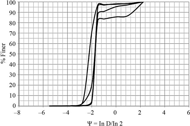
Grain-size distributions for sediment collected during 2010 using the Helley-Smith sampler are shown in Figure 4. No data are available for samples collected in 2009, because they were inadvertently misplaced. The horizontal scale in the figure is given in the Ψ scale [35], which is defined as lnD/ln2, where D is the diameter in millimeters. An analysis of results reveals three distinctive types of sediments: 1) nearly uniform fine sand; 2) bimodal distributions containing fine sand and medium gravel; and 3) medium gravel. Samples gathered on 24 June contain sediment type 1). Samples taken on 28 July, 26 August, and 23 September show the coexistence of sediment types 1) and 2). Samples collected on 9 August indicate the presence of sediment types 1) and 3).
Well-defined dunes with small superimposed dunes characterized the riverbed in an area located upstream of the river bend. Figure 5 shows some of the bed forms detected on 23 September 2010. The geometric dimensions of dunes and small superimposed dunes were measured, and steepness ratios were calculated. In general, dune wavelength increased with increasing discharge.
Table 2. Suspended sediment concentrations and bed sediment loads.
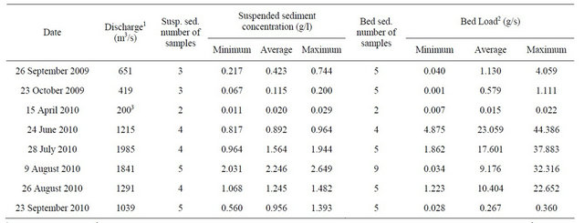
1USGS reported values; 2Point value, from the Helley-Smith sampler, calculated as the ratio between dry sediment weight and sampling time; 3Ice-covered conditions, data collected by UAF crew.
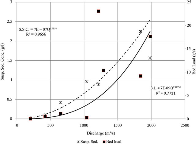
Figure 3. Sediment rating curves. Trend lines represent power distributions. Dashed and solid lines correspond to suspendedsediment concentration and bed load, respectively.
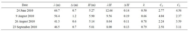
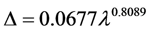
Average values were 67, 56, 41, and 46 m on 24 June, 9 August, 26 August, and 23 September, respectively. Additional geometric characteristics of dunes are provided in Table 3. Average values of small-superimposed dune wavelength ranged from 13 to 16 m. Additional geometric characteristics of small superimposed dunes are given in Table 4. Computed minimum, average, and maximum steepness ratios are provided in Table 5. Results indicate that small superimposed dunes are always steeper than dunes. Figure 6 shows the temporal variation of river discharge and the average values reported in Table 5. Figure 7 shows velocity distributions, collected by the ADCP, along river cross sections located in the proximity of the area where dunes were found.
Finally, calculated water-surface slope, S, for the study reach on 9 August 2010 was 0.00019.
6. Discussion
As described previously (see Table 2), the variation in suspended-sediment concentration along the thalweg in the river reach is relatively small, while the variation in bed load is big, in spite of the fact that sediment sampling was limited in terms of number of samples and location. These results agree with findings previously published [1,20,36,37].
The ADCP-generated measurements of channel area, width, and velocity (see Figure 7) were used to calculate the Froude number given by the following equation:
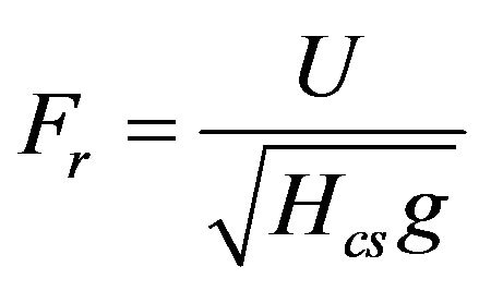 (1)
(1)
where U denotes the cross-sectional average velocity and g denotes gravity. The average cross-sectional depth is obtained as
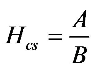 (2)
(2)
where A denotes the cross-sectional area and B denotes the channel width. Calculated Froude numbers were 0.21, 0.23, 0.21, and 0.24 for 24 June, 9 August, 26 August, and 23 September, respectively.
In addition, the dimensionless wave-number, k, [1] was calculated as
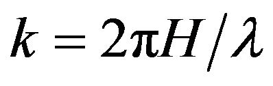 (3)
(3)
where H denotes the average water depth over dunes. Wave-number values were 0.5 - 0.79 (see Table 6), which were in the range of reported values [1]. These numbers and Froude numbers were plotted in a phase diagram for dunes and antidunes based on linear potential theory (see Figure 2.37 on page 83 in [1]). The points fall in the lower area of the graph where dunes are possible. Thus, the field data are in agreement with a previously
 (a)
(a)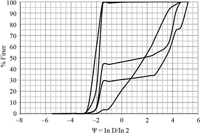 (b)
(b)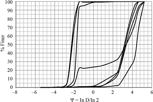 (c)
(c)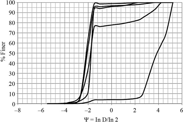 (d)
(d)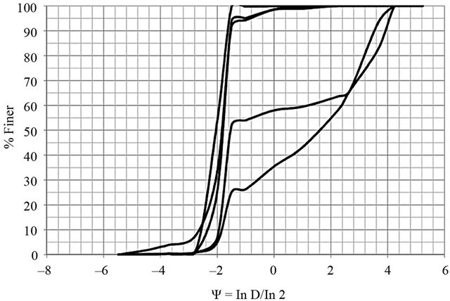 (e)
(e)
Figure 4. Sediment grain-size distributions along the study reach. (a) 24 June; (b) 28 July; (c) 9 August; (d) 26 August; (e) 23 September.
published theory.
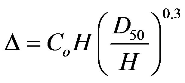
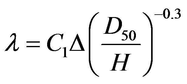
Julien and Klaassen [38] reported the following relationships for dune height and wavelength:
 (4)
(4)
 (5)
(5)
where D50 denotes the median grain size, and Co and C1 denote coefficients ranging from 0.8 to 8 and 0.5 to 8, respectively. Calculated values for these coefficients,
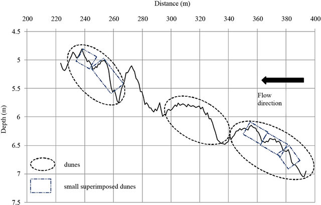
Figure 5. Bed forms surveyed on 23 September 2010.
Table 3. Geometric dimensions of dunes.
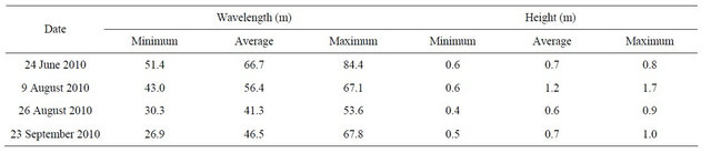
Table 4. Geometric dimensions of small superimposed dunes.
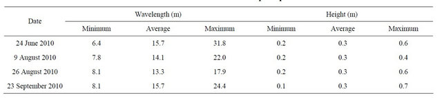
Table 5. Steepness ratio of dunes and small superimposed dunes.
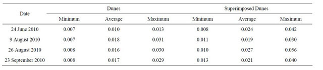
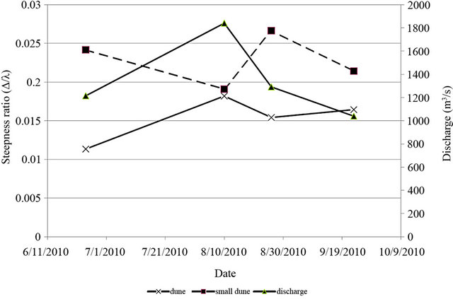
Figure 6. Temporal variation of river discharge and dune steepness ratio.
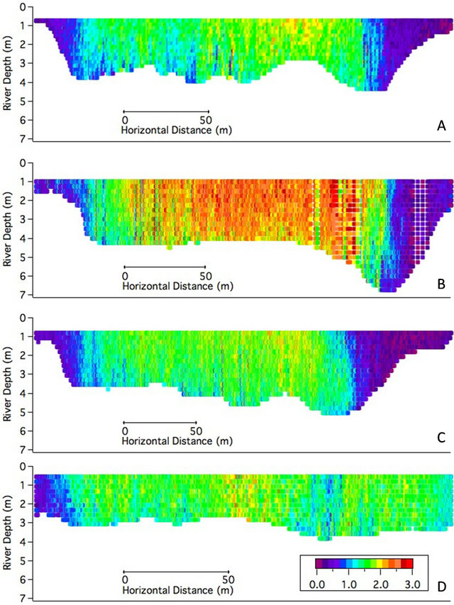
Figure 7. Velocity distributions along river cross-sections. A: 24 June 2010; B: 9 August 2010; C: 26 August 2010; D: 23 September 2010. Cross-sections are viewed looking downstream with left bank on the left-hand side. Velocities are in m/s.
Table 6. Dune parameters and coefficients for different relationships.
based on average data gathered in the Tanana River, ranged from 2.24 to 4.04 and from 2.37 to 4.56 (see Table 6). Thus, the calculated coefficients are in the range of reported values [38].
Bridge [39]—see original work done by Ashley [40]— reported the following empirical relationship for dune height as a function of the wavelength:
 (6)
(6)
It was found that Equation (6) consistently overpredicted the dune height by a factor of approximately two. Thus, Equation (6) should not be applied to the study area. However, the data agree with the graphs reporting λ and Δ as a function of water depth (see Figure 4.13 on page 88 in [39]).
Data indicate that the ratio λ/H (Table 6 and Figure 2) during rising stages is higher than during receding stages. In addition, the ratio Δ/H (Table 6) generally agrees with reported values: Δ/H ≤ 1/6 [1].
The riverbed characteristic (i.e., dunes with small superimposed dunes) is similar to bed configurations found in other large alluvial rivers (see, for instance, details provided in Chapter 2, [1]). Dune and small-dune wavelengths on the study reach are comparable to analogous bed forms reported on Rhine River branches in The Netherlands [41]. Small dunes are consistently steeper than dunes, which is in agreement with published data [42]. The temporal evolution of dune steepness and discharge (Figure 6) also agrees with trends found in the Rhine River [38].
Table 3 indicates that the percentage of change for average wavelengths and dune heights, which are defined here as 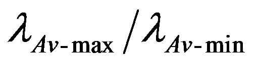 and
and , are 61% and 100% for wavelength and height, respectively. The same ratios were calculated for the small superimposed dunes (Table 4). Obtained results were 18% and 0% for wavelength and height, respectively. Thus, one could argue that in the case of dunes, height controls the steepness ratio; while in the case of small superimposed dunes, wavelength controls the steepness ratio.
Available sediment grain-size distributions indicate that nearly uniform fine sand (see Figure 4(a)—24 June 2010) corresponded to the minimum value of average steepness ratio of dunes (Table 5). Furthermore, when the majority of sediment samples were in the medium-gravel ranges (see Figure 4(c)—9 August 2010), the value of average steepness ratio of dunes was maximum (Table 5). Thus, one could argue that some links between sediment sizes and steepness may exist.
The knowledge gained in this work, which is mainly related to geometric dimensions of bedforms, near-bed sediment characteristics, and suspended sediment load, provides basic information for the engineering design of anchoring devices and abrasion of components exposed to the water flow in power generation devices. Specifically, geometric bedform dimensions (wavelength and height) give insights on the variation of bed material coverage for subsurface anchor platforms. Suspended sediment loads provide information for maintenance/replacement operations due to sediment abrasion.
7. Conclusions
This work presents preliminary sediment-rating curves and bed form characteristics of the Tanana River near Nenana, Alaska, USA. Fieldwork efforts focused along the thalweg, where hydrokinetic devices are expected to be deployed. The study site is located at 64˚33'50"N and 149˚04'W. With information from the field and lab, it is possible to report grain-size distributions of sediment moving near the bed as well as the temporal evolution of dune steepness.
Suspended-sediment concentrations are highly correlated with river discharge. The estimated R-squared coefficient is above 0.96, while the same coefficient between local bed load and river discharge is 0.77.
Based on all data collected, one can define the river in the study area as a sand-gravel riverbed, with several types of sediment coexistent in the region: namely, nearly uniform fine sands, fine gravels, and sediment showing a bimodal distribution.
Dunes with small superimposed dunes were found in the center of the river immediately upstream of the river bend. Dune wavelengths ranged from 41 to 67 m, while small-dune wavelengths ranged from 13 to 16 m. Steepness increased a little with increasing discharge. Field data agreed with several published relationships for this type of bed form.
The information provided here can be used for designing anchoring systems and estimating blade abrasion on hydrokinetic devices to be deployed along the study reach.
8. Acknowledgements
I thank Jack Schmid, Rowland Powers, Ryan Tyler, and Jerry Johnson for conducting the fieldwork and sediment analyses. I would also like to thank Peter Prokein and Paul Duvoy for preparing figures for this article. Data collection efforts were funded by a project supported by the Alaska Energy Authority, under contract 2195437/ G000055721 to the University of Alaska Fairbanks.
REFERENCES
- ASCE, “Sedimentation Engineering: Processes, Measurements, Modeling and Practice,” Manual 110, Reston, 2008.
- W. Brownlie, “Flow Depth in Sand-Bed Channels,” Journal of Hydraulic Engineering, Vol. 109, No. 7, 1983, pp. 959-990. doi:10.1061/(ASCE)0733-9429(1983)109:7(959)
- F. Karim, “Bed-Form Geometry in Sand-Bed Flows,” Journal of Hydraulic Engineering, Vol. 125, No. 12, 1999, pp. 1253-1261. doi:10.1061/(ASCE)0733-9429(1999)125:12(1253)
- N. Marsh, A. Western and R. Grayson, “Comparison of Methods for Predicting Incipient Motion for Sand Beds,” Journal of Hydraulic Engineering, Vol. 130, No. 7, 2004, pp. 616-621. doi:10.1061/(ASCE)0733-9429(2004)130:7(616)
- S. Wright and G. Parker, “Density Stratification Effects in Sand-Bed Rivers,” Journal of Hydraulic Engineering, Vol. 130, No. 8, 2004, pp. 783-795. doi:10.1061/(ASCE)0733-9429(2004)130:8(783)
- R. Millar, “Theoretical Regime Equations for Mobile Gravel-Bed Rivers with Stable Banks,” Geomorphology, Vol. 64, No. 3-4, 2005, pp. 207-220. doi:10.1016/j.geomorph.2004.07.001
- O. Navratil, M. Albert, E. Herouin and J. Gresillon, “Determination of Bankfull Discharge Magnitude and Frequency: Comparison of Methods on 16 Gravel-Bed River Reaches,” Earth Surface Processes and Landforms, Vol. 31, No. 11, 2006, pp. 1345-1363. doi:10.1002/esp.1337
- G. Parker, “Surface-Based Bedload Transport Relation for Gravel Rivers,” Journal of Hydraulic Research, Vol. 28, No. 4, 1990, pp. 417-436. doi:10.1080/00221689009499058
- R. Fernandez, J. Best and F. Lopez, “Mean Flow, Turbulence Structure, and Bedform Superimposition across the Ripple-Dune Transition,” Water Resources Research, Vol. 42, No. 5, 2006, Article ID: W05406.
- J. Best, “The Fluid Dynamics of River Dunes: A Review and Some Future Research Directions,” Journal of Geophysical Research, Vol. 110, No. F4, 2005, Article ID: F04S02. doi:10.1029/2004JF000218
- S. Giri and Y. Shimizu, “Numerical Computation of Sand Dune Migration with Free Surface Flow,” Water Resources Research, Vol. 42, No. 10, 2006, Article ID: W10422.
- A. Baghlani and N. Talebbeydokhti, “A Mapping Technique for Numerical Computations of Bed Evolutions,” Applied Mathematical Modelling, Vol. 31, No. 3, 2007, pp. 499-512. doi:10.1016/j.apm.2005.11.021
- Y. Shimizu, S. Giri, S. Yamaguchi and J. Nelson, “Numerical Simulation of Dune-Flat Bed Transition and Stage-Discharge Relationship with Hysteresis Effect,” Water Resources Research, Vol. 45, No. 4, 2009, Article ID: W04429, doi:10.1029/2008WR006830
- M. Amsler, M. Blettler and I. Ezcurra, “Influence of Hydraulic Conditions over Dunes on the Distribution of the Benthic Macroinvertebrates in a Large Sand Bed River,” Water Resources Research, Vol. 45, No. 6, 2009, Article ID: W06426.
- R. Batalla and J. Martin-Vide, “Thresholds of Particle Entrainment in a Poorly Sorted Sandy Gravel-Bed River,” Catena, Vol. 44, No. 3, 2001, pp. 223-243. doi:10.1016/S0341-8162(00)00157-0
- M. Kleinhans, “The Key Role of Fluvial Dunes in Transport and Deposition of Sand-Gravel Mixtures, a Preliminary Note,” Sedimentary Geology, Vol. 143, No. 1-2, 2001, pp. 7-13. doi:10.1016/S0037-0738(01)00109-9
- P. Wilcock and S. Kenworthy, “A Two-Fraction Model for the Transport of Sand/Gravel Mixtures,” Water Resources Research, Vol. 38, No. 10, 2002, p. 1194.
- M. Kleinhans and L. Van Rijn, “Stochastic Prediction of Sediment Transport in Sand-Gravel Bed Rivers,” Journal of Hydraulic Engineering, Vol. 128, No. 4, 2002, pp. 412-425. doi:10.1061/(ASCE)0733-9429(2002)128:4(412)
- Y. Cui, “The Unified Gravel-Sand (TUGS) Model: Simulating Sediment Transport and Gravel/Sand Grain Size Distributions in Gravel-Bedded Rivers,” Water Resources Research, Vol. 43, No. 10, 2007, Article ID: W10436.
- W. Carey, “Variability in Measured Bedload-Transport Rates,” Water Resources Bulletin, Vol. 21, No. 1, 1985, pp. 39-48. doi:10.1111/j.1752-1688.1985.tb05349.x
- R. Batalla, “Evaluating Bed-Material Transport Equations Using Field Measurements in a Sandy Gravel-Bed Stream, Arbucies River, NE Spain,” Earth Surface Processes and Landforms, Vol. 22, No. 2, 1997, pp. 121-130. doi:10.1002/(SICI)1096-9837(199702)22:2<121::AID-ESP671>3.0.CO;2-7
- M. de Vries, “On Measuring Discharge and Sediment Transport in Rivers,” International Seminar on Hydraulics of Alluvial Streams, Delft Hydraulics Laboratory, New Delhi, 1973, 15 p.
- R. Frings and M. Kleinhans, “Complex Variations in Sediment Transport at Three Large River Bifurcations during Discharge Waves in the River Rhine,” Sedimentology, Vol. 55, No. 5, 2008, pp. 1145-1171. doi:10.1111/j.1365-3091.2007.00940.x
- C. Rennie and R. Millar, “Measurement of the Spatial Distribution of Fluvial Bedload Transport Velocity in Both Sand and Gravel,” Earth Surface Processes and Landforms, Vol. 29, No. 10, 2004, pp. 1173-1193. doi:10.1002/esp.1074
- W. Emmet, “A Field Calibration of the Sediment Trapping Characteristics of the Helley-Smith Bedload Sampler,” US Geological Survey, Open File Report 79-411, 1979.
- J. Brasington, B. Rumsby and R. McVey, “Monitoring and Modeling Morphological Change in a Braided Gravel-Bed River Using High Resolution GPS-Based Survey,” Earth Surface Processes and Landforms, Vol. 25, No. 9, 2000, pp. 973-990. doi:10.1002/1096-9837(200008)25:9<973::AID-ESP111>3.0.CO;2-Y
- K. Bunte, S. Abt, J. Potyondy and S. Ryan, “Measurement of Coarse Gravel and Cobble Transport Using Portable Bedload Traps,” Journal of Hydraulic Engineering, Vol. 130, No. 9, 2004, pp. 879-893. doi:10.1061/(ASCE)0733-9429(2004)130:9(879)
- D. Rickenmann and B. McArdell, “Continuous Measurement of Sediment Transport in the Erlenbach Stream Using Piezoelectric Bedload Impact Sensors,” Earth Surface Processes and Landforms, Vol. 32, 2007, pp. 1362- 1378.
- D. Rickenmann, J. Turowski, B. Fritschi, A. Klaiber and A. Ludwig, “Bedload Measurements at the Erlenbach Stream with Geophones and Automated Basket Samplers,” Earth Surface Processes and Landforms, Vol. 37, No. 9, 2012, pp. 1000-1011. doi:10.1002/esp.3225
- D. Wren, S. Bennett, B. Barkdoll and R. Kuhnle, “Studies in Suspended Sediment and Turbulence in Open Channel Flows,” US Department of Agriculture, Research Report 18, 2000, 133 p.
- H. Toniolo, P. Duvoy, S. Vanlesberg and J. Johnson, “Modeling and Field Measurements in Support of the Hydrokinetic Resource Assessment for the Tanana River at Nenana, Alaska,” Proceedings of the Institution of Mechanical Engineers. Part A: Journal of Power and Energy, Vol. 224, No. 8, 2010, pp. 1127-1139.
- T. Brabets, B. Wang and R. Meade, “Environmental and Hydrologic Overview of the Yukon River Basin, Alaska and Canada,” US Geological Survey Water-Resources Investigations Report 99-4204, Anchorage, 2000.
- ASTM, “Standard D3977-97,” 2009. www.astem.org
- ASTM, “Standard C136-06,” 2010. www.astem.org
- G. Parker and D. Andrews, “Sorting of Bed Load Sediment by Flow in Meander Bends,” Water Resources Research, Vol. 21, No. 9, 1985, pp. 1361-1373.
- J. Pitlick, “Variability of Bed Load Measurement,” Water Resources Research, Vol. 24, No. 1, 1988, pp. 173-177.
- M. Kleinhans and W. Ten Brinke, “Accuracy of CrossChannel Sampled Sediment Transport in Large SandGravel-Bed Rivers,” Journal of Hydraulic Engineering, Vol. 127, No. 4, 2001, pp. 258-269. doi:10.1061/(ASCE)0733-9429(2001)127:4(258)
- P. Julien and G. Klaassen, “Sand-Dune Geometry of Large Rivers during Floods,” Journal of Hydraulic Engineering, Vol. 121, No. 19, 1995, pp. 657-663. doi:10.1061/(ASCE)0733-9429(1995)121:9(657)
- J. Bridge, “Rivers and Floodplains: Forms, Processes, and Sedimentary Record,” Blackwell Publishing, Malden, 2003.
- G. Ashley, “Classification of Large-Scale Subaqueous Bedforms: A New Look at an Old Problem,” Journal of Sedimentary Research, Vol. 60, No. 1, 1990, pp. 160-172. doi:10.2110/jsr.60.160
- P. Julien, G. Klaassen, W. Ten Brinke and A. Wilbers, “Case Study: Bed Resistance of Rhine River during 1998 Flood,” Journal of Hydraulic Engineering, Vol. 128, No. 12, 2002, pp. 1042-1050. doi:10.1061/(ASCE)0733-9429(2002)128:12(1042)
- M. Amsler and M. Garcia, “Discussion of Sand-Dune Geometry of Large Rivers during Floods by P. Y. Julien and G. J. Klaasen,” Journal of Hydraulic Engineering, Vol. 123, No. 6, 1997, pp. 582-584. doi:10.1061/(ASCE)0733-9429(1997)123:6(582)
Notations
The following symbols were used in this article:
A: cross-sectional area;
B: channel width;
C: suspended-sediment concentration;
Co, C1: empirical coefficients;
D: sediment diameter;
D50: median sediment size;
FR: Froude number;
H: average water depth over dunes;
Hcs: average cross-sectional water depth;
k: wave-number;
Q: discharge;
Qsb: total bed load;
Qss: total suspended load;
U: cross-sectional average velocity;
S: water-surface slope;
Δ: dune (small superimposed dune) height;
ΔAv-max: maximum value of average dune (small superimposed dune) height;
ΔAv-min: minimum value of average dune (small superimposed dune) height;
λ: dune (small superimposed dune) wavelength;
λAv-max: maximum value of average dune (small superimposed dune) wavelength;
λAv-min: minimum value of average dune (small superimposed dune) wavelength;
Δ/λ: steepness;
Ψ: sediment scale, which is defined as lnD/ln2.