Modern Mechanical Engineering
Vol.06 No.04(2016), Article ID:72449,22 pages
10.4236/mme.2016.64013
A Statistical Theory of the Damage of Materials
Georgi Zachariev
Bulgarian Academy of Sciences, Sofia, Bulgaria

Copyright © 2016 by author and Scientific Research Publishing Inc.
This work is licensed under the Creative Commons Attribution International License (CC BY 4.0).
http://creativecommons.org/licenses/by/4.0/


Received: June 20, 2016; Accepted: November 27, 2016; Published: November 30, 2016
ABSTRACT
A statistical theory of disperse damage of materials gained under loading is proposed. It is based on the idea of distribution of potential damage spots within a specimen similar to the distribution of the strength values found by testing a set of identical specimens. A relation between damage risk and the probability of damage of a single specimen is assumed. It conforms to the relation between risk and probability of strength distribution of a set of identical specimens, according to Weibull’s statistical theory of material strength. The damage risk just like the damage probability are assumed to be functions of loading and time. Damage is modeled regarding two mechanisms―thermo-fluctuation damage based on the kinetic theory of material strength, and damage depending on a parameter called loading degree (percentage), which depends on load and time. The first mechanism adopts two relations regarding energy barrier reduction due to loading. Equations of damage advance under short-term loading (with a constant rate of load increase) and under long-term (constant) loading are derived. Theoretical relations of damage development are compared with experimental evidence gained via specific tests on short glass fibre reinforced polyoximethylene. The damage itself consists of the accumulation of additional internal surfaces within the entire material volume as measured by small angle scattering X-ray refractometry. It is shown that the mechanism of damage as a function of loading degree where time participates implicitly, gains advantage over the kinetic mechanism where time is explicitly present. The cumulative functions derived for damage accumulation can be used to assess not only damage, but also for statistical analysis of the strength and other quantities.
Keywords:
Damage Mechanics, Mechanical Testing, Non-Destructive Testing

1. Introduction
Two mechanical processes proceed in materials under loading: deformation and fracture. Whereas the deformation can be measured on any kind of basis, the registration of fracture kinetics is a much more difficult problem. This is the reason why one would perform mechanical investigations, usually assessing not the fracture process itself but recording such integral values as strength and time to fracture―results of fracture development. This is also the reason for the introduction of some internal parameter whose physical meaning is not clear but which is to describe the damage process. Note however that there are other approaches which indirectly assess damage by registering the change of some mechanical or geometrical macrovalues, i.e. also without clear physical meaning.
The aim of this work is to derive equations approximating the damage process. Under damage we shall understand the accumulation of additional internal surfaces (micro, mezzo and macro cracks, debondings, pores) in the entire material volume due to the loading i.e. the dispersed damage in our work has a clear physical meaning. A statistical theory is developed for that purpose. The idea of Weibull for a connection between risk and probability of fracture is used. A damage model is proposed where these two quantities are assumed to be functions of loading and time. It is also assumed that potential places (spots) of damage exist within the entire material volume. Two mechanisms of spot fracture are investigated: A thermo-fluctuation one and a mechanism where spot fracture is determined by an especially defined parameter.
2. Damage Model
The notable researcher W. Weibull, in his work on strength of materials published in 1939 [1] , made no other assumption but that there exists a cumulative function of the distribution of the strength of identical specimens. Its derivative with respect to strength is the distribution function. Furthermore, Weibull concluded that “it is obvious that the distribution curve should not be influenced and distorted by alien factors independent of the specimen itself, as for instance method of measurement, measuring instruments, fixation of the test specimens, etc., but that it should be an expression of the strength properties of the material”.
A key point of Weibull’s theory is the introduction of the term “risk of rupture” R (referred to as “risk” for brevity in what follows), involving a cumulative function of strength distribution W (Weibull denoted quantities R and W, depending on strength , by B and S, respectively, in his work). The link between R and W is given by the equation:
 (1)
(1)
Function  is the probability of specimen fracture at stress
 . Here a natural logarithm is used instead of a common logarithm used in [1] .
Assume that damage develops due to the existence of different potential places― spots in the material, which become active (i.e. unleash damage) depending on stress  and time t. Assume also a link between risk of damage
  and damage probability
  in a form identical to that in (1):
 (2)
(2)
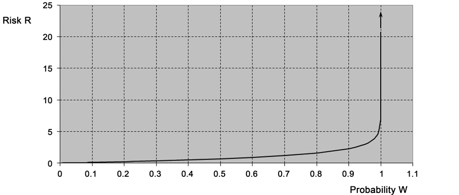
Regardless of whether we consider strength or damage, the dependence between risk R and probability W is ―see Figure 1(a). For zero probability W, risk R is also zero while for
  (i.e. 100% probability) risk
For low probability, risk R is approximately equal to probability W, i.e. R ≈ W (Figure 1(b)).
Despite the identical forms, Equations ((1) and (2)) significantly differ from each other: Equation (1) presents the distribution of strength of a set of identical specimens while Equation (2) sets forth the distribution of damage spots within the material, i.e.
 (a)
(a)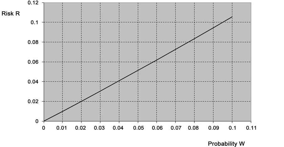 (b)
(b)
Figure 1. (a) Dependence of the risk R on the probability W; (b) dependence of the risk on the probability at ;
; .
.
within each specimen.
Assume the following relation for damage :
:
 (3)
(3)
where  is the maximal possible damage when all potential damage spots are activated i.e. fractured.
Consider two loading types: short-term loading with constant rate of stress increase and long-term loading with constant stress (so called regime of creep).
Time and load can be introduced in risk  based on two mechanisms of spot fracture:
- a thermo-fluctuation mechanism where heat fluctuations play a decisive role in damage occurrence (spot fracture);
- a mechanism where spot fracture is determined by a parameter depending on time, load and rate of load increase;
3. Thermo-Fluctuation Mechanism of Damage (Mechanism I)
The thermo-fluctuation mechanism of damage lies within the basis of the kinetic theory of fracture [2] , developed in the Ioffe institute (St Petersburg―Russia). According to this theory heat fluctuations play a major role in damage accumulation. Mechanical stress only decreases the energy barrier that heat fluctuations should overcome to instigate fracture.
Ref. [2] treats break of an interatomic bond with an energy barrier  to be overcome by the fluctuations, thus yielding fracture.
  is the energy barrier in non-loaded state,
  is decrease of
  due to loading (stress
 ). Heat fluctuations are of probabilistic character. For the mean statistical “life” of the interatomic bond
 , i.e. for its mean statistical time to fracture is assumed that:
 (4)
(4)
where  is a constant whose value is close to that of the period of atom thermal oscillations; h―Planck’s constant; k―Boltzmann’s constant;T―absolute temperature.
Based on break of the interatomic bonds, we assume the following model of damage accumulation: there exist potential damage spots in the material having identical energy barriers . Here, the energy barrier in non-loaded state
  and its decrease due to loading
 , as well as all other quantities refer to damage spots and not to interatomic bonds.
Thermal fluctuations with energy  are needed for spot fracture, i.e. for damage initiation and generation, and the values of
  are discrete and divisible by
 . The higher
  of the expected fluctuation, the longer the mean statistical period
  of fluctuation occurrence.Assume the relation:
 (5)
(5)
where  for spots is constant like
  in (4) for an interatomic bond.
The hazardous heat fluctuations, i.e. those yielding fracture of spots, read:
 (6)
(6)
The frequency of occurrence of hazardous fluctuations is  where
where  assumes values following (6).
The total frequency of the occurrence of hazardous fluctuations  is a sum of the frequencies of occurrence of fluctuations with energy
  following (6):
 (7)
(7)
where  and e is the base of the natural logarithms.
It follows from (7) that the account for all possible hazardous heat fluctuations increases the frequency of damage generation by .
.
Assume that risk  is proportional to time t and to the frequency of occurrence of hazardous fluctuation
 .
.
Considering (5) and (7), it follows for long-term loading (σ = const.) that:
 (8)
(8)
Assume for , which is a constant quantity in this case, that:
 (9a)
(9a)
or
 (9b)
(9b)
Pursuant to (9a)  corresponds to
  and
and ― to
― to , while
  corresponds to the structurally sensitive coefficient of the kinetic theory of fracture [2] .
According to (9a) we have for :
:
 (8a)
(8a)
where  and
and .
.
According to (9b) we have for  in (8):
 (8b)
(8b)
where  and
and .
.
Consider a short time of stress increase with a constant rate . Assume that stress keeps constant for each infinitesimally short period of time
 . Accounting for (8), we find the following relation for risk:
 (10)
(10)
For , following (9а), i.e.
 :
:
 (11)
(11)
For , following (9b), i.e.
 :
:
 (12)
(12)
4. Damage as Dependent on a Specified Loading Parameter (Mechanism II)
Assume a mechanisms of damage where damage spot activation (i.e. spot fracture and damage generation) takes place depending on a specific loading parameter p. Assume also that a curve of spot distribution exists, which is a function of that parameter: some spots fracture under smaller values of p, while others―under larger values of p.
Adopt loading degree (percentage) as a loading parameter, defined as follows:
- for short-term loading (index K) under constant stress rate :
:
 (13)
(13)
where  is strength at rate of stress increase
  and t is time.
- for long-term loading (index L) under constant stress :
:
 (14)
(14)
where  is the long-term strength and
  is durability, i.e. time to macrofracture.
Assume a linear relation between the long-term strength and the logarithm of durability, i.e.:
 (14a)
(14a)
where a and b are coefficients.
The degree of loading p specifies a relation between stress acting at a specific time and material fracture stress regarding the same conditions (i.e. rate of stress increase during short-term loading and time of stress application during long-term loading). It follows from (13) and (14) that p is a function of time for both loading types.
As for the function of the risk of damage  one may assume either a power form (similar to the rupture risk in [1] ), or an exponential form:
 (15)
(15)
 (16)
(16)
where  and
and  are coefficients.
The choice of a power or exponential form of risk  is based on the concave form of the cumulative function of damage accumulation during the initial stage, which is experimentally found. The same holds true for the risk of rupture in Weibull’s theory where not only a power ( [1] ) but also an exponential form of risk
  may be adopted conforming to (1).
5. Functions of Damage Accumulation
The cumulative functions of damage  conforming to the adopted mechanisms are found based on damage probability W and risk R:
 (17)
(17)
The accuracy of the approximation in (17) is as greater as  is smaller than
 .
.
Mechanism I
Short-term loading :
:
? with R following (11):
 (18)
(18)
where
 (18')
(18')
? with R following (12):
 (19)
(19)
where
 (19')
(19')
Long-term loading :
:
? with R following (8) and (9а):
 (20)
(20)
? with R following (8) and (9b):
 (21)
(21)
Consider relations (20) and (21) and a macrofracture criterion stating that fracture occurs when critical damage  is attained (
 ). Then, the following relations between the constant stress
  and durability
  are found:
according to (20):
 (20')
(20')
according to (21):
 (21')
(21')
where:


i.e. linear relations between the durability logarithm and the constant stress (its logarithm, respectively) are derived.
Mechanism II
Consider both loading types (long-term and short-term ones) and relations (17), (15) and (16). Then, it follows that:
 (22)
(22)
 (23)
(23)
where p is presented by (13) for short-term loading, and by (14)-for long-term loading.
The comparison between the cumulative functions of damage, considering both mechanisms, shows the following specificities:
- Functions  according to mechanism I differ from each other for short-term and long-term loadings (compare (18) and (19) to (20) and (21)). Yet, they are identical for the same loadings according to mechanism II (see (22) and (23)).
- Functions  for short-term loading, regarding both mechanisms, are similar with respect to time
  in (18) and (19) and loading degree
  in (22) and (23). The difference lies in the explicit presence of
  and
and  in (18) and (19), while
  and
and  are implicitly present in (22) and (23) through the degree of loading
 , according to (13).
- The assumption of the form of  according to (9а) and (9b) specifies the respective exponential (see (18)) or power (as in Weibull, see (19)) form of the relations for damage accumulation.
To compare damage accumulation found pursuant to both mechanisms, we shall present  according to mechanism I as a function of the loading degree
  in (18), (19), (20) and (21), using relations (13), (14), (20') and (21'):
 (18a)
(18a)
where:
 (18a')
and  and
and  are according to (18').
 (19a)
(19a)
where:
 (19aʹ)
and  and
and  are according to (19').
The cumulative function (19а), as well as that in (19) are similar to Weibull’s function, but having parameters depending on .
.
 (20a)
(20a)
where  and
and  are coefficients in Equation (20') for the long-term strength.
 (21a)
(21a)
where  and
and  are coefficients in Equation (21') for the long-term strength.
6. Experimental Verification of the Cumulative Functions
The experimental verification of the cumulative functions pursuant to mechanism I- (18а), (19а), (20а), (21а) and mechanism II-(22) and (23) requires the performance of specially designed experiments in order to register damage development for both loading regimes-short-term and long-term ones.
Assume that damage  is due to the activated i.e. fractured damage potential sites, herein referred to as damage spots. Fractured spots, on their part, are in correspondence with the internal surfaces formed within the material volume as a result of loading. The internal surfaces are measured using an unconventional small angle X-ray refraction method developed by M.P. Hentshel and collaborators [3] [4] in the Federal Institute of Materials Research and Testing (BAM―Berlin, Germany). The measure of damage is the difference between the refraction of loaded-unloaded samples and the refraction of a virgin sample. Tests are performed on a material allowing the application of Hentshel’s method of damage registration. The results are published in [5] [6] [7] . We present here a brief description of the experimental technique and the results found using them to assess the validity of the derived cumulative functions.
6.1. Material
The material is injection moulded polyoximethylene reinforced by means of short glass fibers. Samples, produced by Ticona GmbH Frankfurt a.M. in compliance with DIN EN ISO 527, are characterized with glass fibre (E-glass) part 26 wt%, mean fibre length 320 μm (max. 800 mm, min. 60 mm) and fibre diameter 10 ± 1 μm. Silane compounds are used for fiber adhesion dressing.
6.2. Mechanical Loading
Samples for a short-term tests were subjected to tension on an Instron testing machinery. Tension was parallel to the oriented short fibres, applying three constant loading rates dF/dt = 0.22; 1.1 and 5.5 [kN/min] i.e. 0.093; 0.465 and 2.326 [MPa/sec] respectively. After attaining different loading steps―50%, 70%, 80%, 85%, 90%, 93%, 95%, 97% and 98% of the force-at-fracture , samples were instantly unloaded. Three samples were used in every step, as well as to measure the initial strength. Experiments were carried out at room temperature and 50 % humidity.
Samples for a long-term tests are loaded by constant tension, using lever loading devices type “Frank”. Load is uniformly fed via a hydraulic jack until attaining a specific value.
To find material long-term strength, time prior to sample fracture is measured applying the following constant loads: 71.88 [MPa]; 82.32 [MPa]; 92.75 [MPa]; 100.6 [MPa]; 108.3 [MPa]. Three samples are tested under each load.
The process of creep damage accumulation is experimentally investigated for 3 degrees of constant loading: 64.06 [MPa], 74.56 [MPa] and 82.24 [MPa], and within three samples per each load. After 2 [h], 4 [h], 6 [h], 24 [h] and 48 [h], respectively, samples are unloaded and accumulated damage is measured.
6.3. Damage Processes and Their Measurement
Damage processes develop in two directions: accumulation of micro and mezzo cracks perpendicular to loading (Figure 2(b)) and accumulation of micro and mezzo fibre/matrix debondings parallel to the loading direction (Figure 2(a)). Damage takes place into the whole material volume. In what follows we denote the two kinds of damage as cracks and debondings, respectively. A damage process proceeds relatively homogeneously in isolated volumes until there is interaction between them and than it spreads to the macrovolume leading to collapse (i.e. to material splitting caused by a macrocrack).
The method of damage measure uses the effect of refraction at very small angles of few arc minutes. The scattered intensity of this refraction is by several magnitudes higher than that of conventional X-ray scattering (diffraction at larger angles).
The internal surfaces inherent to the two types of damage are measured by an appropriate guidance of the X-ray beam (Figure 2(a), Figure 2(b)). In the both cases the scattering plane (the plane determined by the collimated beam and the refracted one) is perpendicular to the plane of the inner surfaces. The planes of cracks are also perpendicular to the loading direction (Figure 2(b)), those of debondings are parallel to it (Figure 2(a)).
Quantity  denotes the refraction factor proportional to the inner surface density (ratio surface S/volume V), k is a constant of the instrument and d is the sample thickness. The three left topogramms in Figure 3 and the three right topogramms in Figure 4 refer to the refraction of three loaded and then instantly unloaded samples, the right topogramm on Figure 3 and the left topogramm on Figure 4 refer to the refraction of a never loaded (virgin) sample. The virgin sample measurements serve as a bench mark for calculating the internal surfaces (damage) having occurred as a result of loading. Damage in each microvolume, fixed by the sample thickness d and the cross section of the X-ray beam, is the difference Δcd between the refractions measured on loaded-unloaded and virgin samples. The different height of the topograms at separate microvolumes and its varying color in Figure 3 and Figure 4 illustrate the distribution

Figure 2. An X-ray beam with cross section 3 mm/50 μm scans an area 10 mm/20 mm, with a horizontal step 1 mm and vertical step 0.2 mm. So the next measurement partially overlaps the previous one. As an example, Figure 3 and Figure 4 show the distribution of single refractions cd measured by scanning loaded-unloaded samples and applying up to 98% of the fracture load, as well as refraction distribution in a virgin sample.

Figure 3. X-ray refraction topograms of loaded-unloaded up to 98% of fracture load samples and virgine sample.  is the damage
  and corresponds to the internal surfaces―cracks.

Figure 4. X-ray refraction topograms of loaded-unloaded up to 98% of fracture load samples and virgine sample.  is the damage
  and corresponds to the internal surfaces―debondings.
of damage within the volume corresponding to the scan area. All measurements shown in each of these figures are included in only one point of diagrams that follow―namely loading step 98% of the force-at-fracture. The same procedure was done for every loading step. Damage was registered by Mr. Heinz Ivers in the Federal Institute of Materials Research and Testing (BAM―Berlin).
The mean arithmetic value of the differences  for three loaded-unloaded samples is assumed as damage ω at every loading step, i.e.:
 (24)
(24)
where m is the mean value of c.
The mean value  implies 1000 single measurements per sample. It corresponds to the mean value of the internal surfaces that arise under loading: cracks and debondings. We shall denote damage corresponding to the inner surfaces oriented perpendicularly to the loading direction (Figure 2(b)) by
 , and those oriented parallel to the loading (Figure 2(a))―by
 . So, the summarized damage corresponding to the summarized accumulation of internal surfaces that arise into the sample volume was measured.
6.4. Experimental Results
Damage accumulation  in two directions for the short- and long-term loading as a function of loading degree (percentage) p is shown in Figure 5 for
  (cracks, i.e. crosswise damage according to Figure 2(b)) and in Figure 6 for
  (debondings, i.e. lengthwise damage according to Figure 2(a)). Damage
  is in relative units, loading degree p (the ratio between the actual stress and the strength) is in percents.
Strength depends on the loading rate: it is 115.94 [MPa] at 0.093 [MPa/sec], 124.19 [MPa] at 0,465 [MPa/sec] and 127.72 [MPa] at 2.326 [MPa/sec], i.e. it increases with the loading rate.
It follows from Figure 5 and Figure 6 that the higher the loading degree, the higher the damage. However, this is to be expected. It can be assumed also from these figures that damage depends on the loading degree, only, but not on the loading type―short- or long-term loading. Damage measured after macrofracture at loading rate 0,465 [MPa/sec] and under short-term loading is denoted by + (cross) in Figure 5 and Figure 6. Damage

Figure 5. Experimental data of damage  (cracks) at short- and long-term loading as a function of loading percentage p.

Figure 6. Experimental data of damage  (debondings) at short- and long-term loading as a function of loading percentage p.
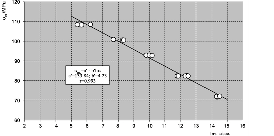
Figure 7. Long-term strength  as a function of the logarithm of time to fracture
  in creep.
values are less than the extrapolated ones at p = 100% according to measurements on unloaded samples. This fact can be explained with the explosion-like unloading at macrofracture, which is different from the unloading at other experimental points. It causes a greater damage closure.
Long-term strength in creep as a function of specimen lifetime (time to fracture) according to Equations ((20') and (21')) is shown in Figure 7 and Figure 8.
6.5. Approximation of Damage According to Mechanism I
Equations ((18a) and (19a)) describe damage accumulation under short-term loading,
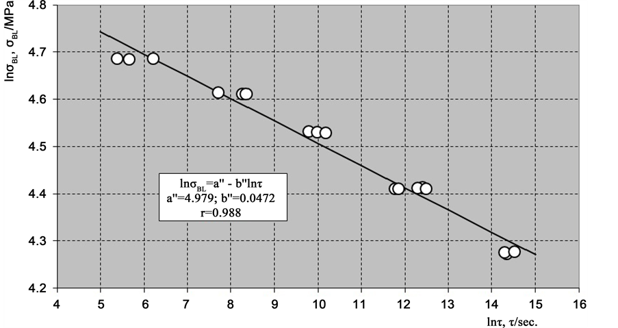
Figure 8. Logarithm of the long-term strength  as a function of the logarithm of the time to fracture
  in creep.
while Equations ((20a) and (21a))―that under long-term loading. There are two coefficients to be determined in these equations:
 and
and  in (18a) and (20a) and
  and
and  in (19a) and (21a). The coefficients were found applying a regression of damage data under short-term loading with a fixed loading rate:
  [MPa/sec] and corresponding strength
  [MPa]. For coefficients with index' the regression is an exponential one with iteration as outlined in [5] , while for those with index" it is a power one.
Figure 9 and Figure 11 show regression results for cracks and debondings respectively. For other loading rates and their corresponding strength, damage accumulation is calculated according to Equations ((18a) and (19a)) and plotted by solid and dashed lines respectively. Index K denotes short-term loading, index L―long-term one.
It follows from Figure 9 and Figure 11, that the calculated damage at  and 0.093 [MPa/sec] as a function of loading degree does not agree with the experimental data.
Figure 10 and Figure 12 show approximations of damage accumulation under long-term loading for cracks and debondings respectively. Solid lines present approximations according to Equation (20a) and dashed ones―according to Equation (21a). The coefficients ,
,  in (20a) as well as
 ,
,  in (21a) were found from short-term tests as explained above (see Figure 9 and Figure 11). The coefficients
 ,
,  in (20a) as well as
 ,
,  were found from relations “lifetime - long-term strength” (see Figure 7 and Figure 8).
It follows from Figure 10 and Figure 12 that the calculated damage presented as a function of loading degree at four constant stresses does not agree with the experimental data.
6.6. Approximation of Damage According to Mechanism II
Equations ((22) and (23)) describe damage accumulation under short- and long-term loading. Loading degree in these equations is calculated according to (13) for short- term loading and according to (14)―for long-term loading.
Figure 13 and Figure 14 show approximations of all experimental data for cracks, while Figure 15 and Figure 16―data approximations for debondings. The coefficients in (22) were found performing an exponential regression with iteration, while those in (23)―performing a power regression.

Figure 9. Damage  at short-term loading (cracks) as a function of loading percentage p.

Figure 10. Damage  at long-term loading (cracks) as a function of loading percentage p.

Figure 11. Damage  at short-term loading (debondings) as a function of loading percentage p.
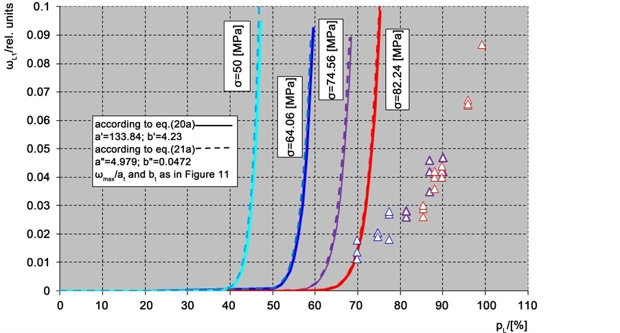
Figure 12. Damage  at long-term loading (debondings) as a function of loading percentage p.

Figure 13. Damage  at a short-term loading (cracks) as a function of loading percentage p.

Figure 14. Damage  at a long-term loading (cracks) as a function of loading percentage p.

Figure 15. Damage  at a short-term loading (debondings) as a function of loading percentage p.

Figure 16. Damage  at a long-term loading (debondings) as a function of loading percentage p.
It follows from Figures 13-16, that the approximations employing both Equations ((22) and (23)) are very good. Comparison shows that the approximation according to Equation (22) is better (the correlation coefficients are larger) than the approximation according to Equation (23). The same result was found in [7] for damage mean values at every p.
7. Other Applications of the Cumulative Functions
The cumulative functions derived to approximate damage―Equations ((22) and (23)), can also be used in statistical data processing. For that purpose, substitute damage  for median rank G, loading degree p for the corresponding quantity x whose values are processed, and
  for specimen general number corresponding to
 . Then Equations ((22) and (23)) take the form:
 (22')
(22')
 (23')
(23')
Equations ((22') and (23')) may be employed to approximate the cumulative functions of the bending strength of float glass [8] (Figure 17), lifetime of electron tubes [8] (Figure 18) and lifetime of turbine engines [9] (Figure 19). Large correlation coefficients are found.
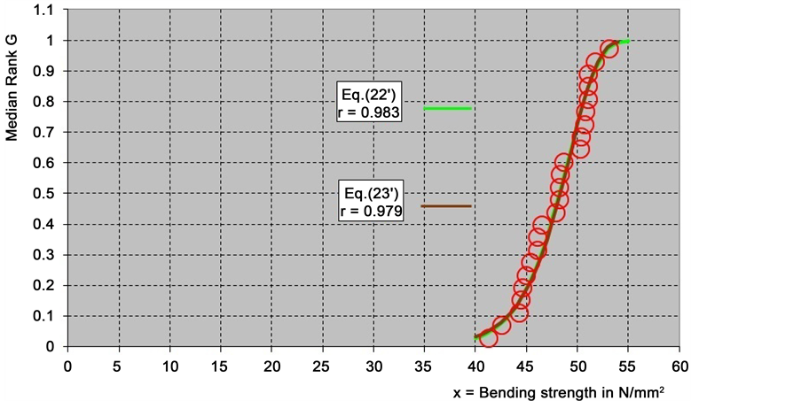
Figure 17. Cumulative distribution function of G. Bending strength of float glass, example 1 from [8] .

Figure 18. Cumulative distribution function of G. Lifetime of electron tubes, example 2 from [8] .

Figure 19. Cumulative distribution function of G. Lifetime of turbine engines, example from [9] .
8. Conclusions
1) A statistical theory of disperse damage of materials gained under loading is proposed. It is based on the idea of distribution of potential damage spots within a specimen similar to the distribution of the strength values found by testing a set of identical specimens. A relation between damage risk and the probability of damage of a single specimen is assumed. It conforms to the relation between risk and probability of strength distribution of a set of identical specimens, according to Weibull’s statistical theory of material strength.
2) Damage is modeled regarding two mechanisms―thermo-fluctuation damage based on the kinetic theory of material strength, and damage depending on a parameter called loading degree (loading percentage), which depends on load and time. The first mechanism adopts two relations regarding energy barrier reduction due to loading. Equations of damage advance under short-term loading (with a constant rate of load increase) and under long-term (constant) loading are derived.
3) Compare the theoretical relations of damage development with experimental evidence gained via specific tests. It is seen that the mechanism of damage as a function of loading degree where time participates implicitly, gains advantage over the kinetic mechanism where time is explicitly present. To approximate damage, one should use Equations ((22) and (23)).
4) It can be assumed, that damage depends on loading degree, only, but not on the loading type (short- or long-term loading). This enables one to predict damage under long-term loading based on data on short-term loading, and vice versa.
5) The cumulative functions (22) and (23) can be used to assess not only damage, but also strength and other quantities.
6) It is necessary to verify the proposed theory for other materials. It provides an opportunity to approximate as well as predict the damage process. The equations derived for damage can be applied to a wide range of cases of material response.
Acknowledgements
This work appears thanks to the financial support of the Alexander von Humboldt Foundation (Bonn, Germany) and the fruitful collaboration with the colleagues from the Federal Institute for Materials Research and Testing (BAM-Berlin, Germany): M. P. Hentshel, H.-V. Rudolph, H. Ivers. I thank my colleagues from the Departament 5, Division 5.3 (Mechanics of Polymers) of the BAM for the long-standing support.
Cite this paper
Zachariev, G. (2016) A Statistical Theory of the Damage of Materials. Modern Mechanical Engineering, 6, 129-150. http://dx.doi.org/10.4236/mme.2016.64013
References
- 1. Weibull, W. (1939) A Statistical Theory of the Strength of Materials. Generalstabens Litografiska Anstalts Förlag, Stockholm.
- 2. Regel, V.R., Slutzker, A.I. and Tomashevskii, E.E. (1974) Kinetic Nature of Strength of Solids. Nauka, Moskow. (In Russian).
- 3. Harbich, H.-W., Hentschel, M.P. and Schors, J. (2001) X-Ray Refraction Characterization of Non-Metallic Materials. NDT&E International, 34, 297-302.
https://doi.org/10.1016/S0963-8695(00)00070-0 - 4. Bullinger, O. (2006) X-Ray Methods in the Field of Non-Destructive Testing and Evaluation of Composite Structures. In: Busse, G., Kröplin, B.-H. and Wittel, F.K., Eds., Damage and Its Evolution in Fiber-Composite Materials: Simulation and Non-Destructive Evaluation, SFB 381, ISD Verlag, Stuttgart, 73-80.
- 5. Zachariev, G., Rudolph, H.-V. and Ivers, H. (2004) Damage Accumulation in Glassfibre-Reinforced Polyoximethylene under Short-Term Loading. Composites Part A, 35, 1119-1123.
https://doi.org/10.1016/j.compositesa.2004.03.018 - 6. Zachariev, G., Rudolph, H.-V. and Ivers, H. (2009) Prediction of Creep-Damage Accumulation in Glass Fibre Reinforced Polyoximethylene. Materials Science and Engineering A, 510-511, 425-428.
https://doi.org/10.1016/j.msea.2008.04.114 - 7. Zachariev, G. (2013) Approximation of Damage Accumulation in Fibre Reinforced Polymers. Materials Testing, 55, 32-37.
https://doi.org/10.3139/120.110408 - 8. DIN 55303-7, March 1996.
- 9. Jensen, F. and Petersen, N.E. (1982) Burn-In. John Wiley & Sons, Chichester, New York, Brisbane, Toronto, Singapore.