Open Journal of Biophysics
Vol.2 No.2(2012), Article ID:18920,6 pages DOI:10.4236/ojbiphy.2012.22006
Age Dependence of the Menstrual Cycle Correlation Dimension
1Physics Department, Loyola University Maryland, Baltimore, USA
2Paula Derry Enterprises in Health Psychology, Baltimore, USA
Email: *gderry@loyola.edu
Received March 13, 2012; revised April 12, 2012; accepted April 19, 2012
Keywords: Perimenopause; Menstruation; Time Series Analysis; Chaos; Correlation Dimension; Menopause
ABSTRACT
Time series analysis, based on the idea that female reproductive endocrine physiology can be construed as a nonlinear dynamical system in a chaotic trajectory, is performed to measure the correlation dimension of the menstrual cycle data from subjects in two different age cohorts. The dimension is computed using a method proposed by Judd (Physica D, vol. 56, 1992, pp. 216-228) that does not assume the correlation dimension to be necessarily constant for all appropriate time scales of the system’s strange attractor. Significant time scale differences are found in the behavior of the dimension between the two age cohorts, but at the shortest time scales the correlation dimension converges to the same value, approximately 5.5, in both cases.
1. Introduction
The typical conceptualization of the menstrual cycle is that it has a stable period of » 28 days throughout most of the reproductive years but becomes irregular and unstable during the perimenopause, i.e. the years preceding the end of menstruation (menopause) [1]. However, the idea that the menstrual cycle is highly regular and periodic not only is discrepant from the experience of many people, it also contradicts a body of published literature [2]. Treloar’s pioneering work [3] demonstrated many years ago that there is significant variability in the human menstrual cycle during the entire life span. Variability increases during perimenopause, but there is controversy in the literature over when this begins and how to characterize it [4-6]. The increased irregularity has often been taken to be evidence of senescence and incipient breakdown in the reproductive system, but given the unexplained variability prior to perimenopause and the lack of any understanding for why such a transition should occur, these interpretations are premature [2]. We have previously hypothesized that the variability in the menstrual cycle is neither random nor extrinsic to the system, but rather is the result of the female reproductive endocrine system being a nonlinear deterministic system in a chaotic trajectory, and we have offered evidence that this is correct [7].
The application of concepts from nonlinear dynamics and chaos to physiological problems has now become well established [8], but relatively little of this work has been performed on the human endocrine system. The collection of concepts and techniques known as time series analysis is one of the primary tools for the treatment of data from nonlinear systems and the characterization of chaos. Successful time series analysis requires sampling an extremely large number of data points, and this is difficult for endocrine studies that typically require much trouble and expense (blood draws, bioassays, etc.) for each point sampled, in contrast to more widely used methods, for example voltage measurements in an electrocardiogram. For this reason, only a relatively small number of time series analyses have been performed using endocrine data, all with considerably fewer than 103 data points and none involving the reproductive system [9-11]. The novel approach that we have developed allows us to study the menstrual cycle and hence the reproductive endocrine system using time series analysis with ~104 data points. In this paper, we employ these techniques, using a different methodological framework from our previous study [7], to make a comparison of menstrual cycle dynamics from women in differing age ranges.
2. Methods
The source of our data is the database maintained by the Tremin Research Program on Women’s Health, which contains the results of an ongoing longitudinal study begun in 1934 [12]. Subjects in this study record the days that they are menstruating, and from this data we can create a sequence of menstrual cycle lengths. Data from a cohort of subjects who participated in the study from when they were 20 years old (or less) until they reached menopause were used in the present work. Data were selected and analyzed separately for two different age ranges: menstrual cycle data from women aged 20 - 40 years, and menstrual cycle data from women during the 6 years preceding menopause. For the older woman data, 130 subjects were used resulting in 8054 menstrual cycle data points. For the younger woman data, a subset of these subjects consisting of 53 women was used resulting in 10,639 menstrual cycle data points. (A different subset of these subjects was used in our previous study [7], so this work also served as a reproducibility check for the 20 - 40 year age range results.) For each age range, the data were analyzed in two different forms. One form was an interevent time sequence consisting of the menstrual cycles themselves (Dti), the other was a formal time series constructed using a novel procedure we have devised. The time series is defined such that fn, the nth term of the time series, is given by the difference between time tn and the time at which the nth menstrual cycle ends. The times tn are equally spaced so that tn = nt where t is the sampling time, giving this scheme the structure of a formal time series. More compactly,
 (1)
(1)
where Dti is the time length of the ith menstrual cycle in the sequence. Though this interevent time sequence itself (the set of Dti) does not meet the requirements of a formal time series, there is good reason to believe that it can be employed in the same manner to characterize chaotic trajectories [13]. Each of these approaches (either using the Dti or using the fn as input data to the time series analysis) makes different assumptions and approximations, so repeating the computations using both of these methods serves as a cross check on the validity of the results. In both cases, a phase space reconstruction (embedding) of the data must be implemented and repeated for a variety of embedding dimensions. Further details concerning this methodology, and a discussion of the issues that arise therefrom, can be found elsewhere [7].
A key concept in nonlinear dynamics and chaos is that the trajectory of the system in a multidimensional phase space of the relevant variables is described by a strange attractor in that space. One of the important quantities used to characterize a chaotic strange attractor is its fractal dimension. Experimentally, the quantity that is frequently calculated to obtain an approximation for this fractal dimension is the correlation dimension of the attractor, which can be computed using a time series of data measured for some system variable. This quantity is defined as
 (2)
(2)
where C(e), the correlation sum, represents the number of interpoint distances in the time series data that are smaller than e. These interpoint distances are computed in an embedding space of dimensionality D greater than that of the correlation dimension itself, with vectors in the embedding space found from sets of points in the time series. A major conceptual problem with this formulation is the presence of the limit, because experimentally there are no data in that limit for a time series of finite resolution. In practice, one can instead use estimators of the correlation dimension, such the Takens estimator [14] computed at a single convenient value of e, or the slope of a log(C) vs. log(e) plot in the scaling region of the data where this plot is linear [15]. We have previously employed these estimators in an analysis of the menstrual cycle data from women in the 20 - 40 year age range [7]. However, the scaling region may not include all the information available about the attractor and does not correspond to the proper e limit in the definition; in addition, the points used in the correlation sums may include correlations due to time rather than to geometry, potentially biasing the results. In this paper, we employ a different estimator due to Judd [16,17], which mitigates some of these disadvantages. Judd has shown, at least for a reasonable class of attractors, that the probability of an interpoint distance being less than e is given by
 (3)
(3)
where d is the correlation dimension of the system. In essence, what Judd has shown is that the effect of not being in the asymptotic limit of e ® 0 is to modify the usual relationship with the multiplication by a polynomial in e. This method then allows us to experimentally fit data over a range of e values and opens the possibility to explore any length (i.e. time) scale dependence that may exist for the correlation dimension d itself.
In practice, the probability P(e), which basically corresponds to the correlation sum, is not used directly. Instead, the number of interpoint distances bi within an interval Dei = ei - ei+1 are counted; such intervals can be referred to as bins. The numbers bi now correspond to the probability pi = Pi - Pi+1 and can be used to find the parameters of Equation (3) for all e smaller than some cutoff value e0. As the cutoff e0 decreases, we approach closer to the asymptotic limit e ® 0, but the number of bin values bi with which to fit the parameters decreases and the fits become problematic. The maximum value of e0 is determined by the fact that the theory is only valid on the decreasing tail of the pi distribution. The correlation dimension d, in this formulation, is not required to be constant for all e0, so in essence we are able to obtain information about how the dimension d varies with the characteristic length scale of the system’s strange attractor by using different values for the cutoff. Judd has shown that the bi have a multinomial distribution, and he suggests fitting the parameters by a log-likelihood maximization of this probability function, but here we instead find the parameters by fitting the data to the probabilities entailed by Equation (3) directly, because we found this procedure to have some advantages in algorithmic speed and stability.
For each of the four cases described above (i.e. younger women using fn; older women using fn; younger women using Dti; older women using Dti), we have computed the correlation dimension for the entire range of accessible e0 cutoffs in embedding dimensions ranging from D = 8 to D = 12. (Computations were also performed in lower embedding dimensions, but these are uninteresting since they merely fill the embedding space; results for D ³ 8 are reported since these values of D should be high enough to obtain valid results for d.) We did not use all of the interpoint distances computable for the N data points available, because that offered no means to check reproducibility, it might bias the results due to time correlations, and it would be computationally inefficient. Instead, for every correlation dimension computed, we sampled random pairs from the population N and used the interpoint distances for those pairs to fill the bins. Using just a few percent of the ~N2 possible pairs provided ample amounts of data in the bins with minimal bias, and this procedure could then be repeated to find out how the random selection affected the consistency of the results. Every case (i.e. selection of D and e0 values) was redone for distributions from three random samplings.
3. Results
An example of the results for a single sampling at a particular value of D and e0 is shown in Figure 1. The bin values are normalized to the total value in all the bins, and the e values are scaled to the cutoff value e0. The best-fit parameters (the correlation dimension d and the three polynomial coefficients in Equation (3) were found by minimizing the sum of the squared differences between the theoretical probability pi and the bin value bi for the set of available ei in each case considered. The case illustrated in Figure 1 is for the time series data of the 20 - 40 year old sample at an embedding dimension of D = 10 and a cutoff value of e0 = 64.2 days, employing 21 ei and bi values in the fit. (Again, note that fewer values become available as e0 decreases, making reliable fits more difficult in the interesting asymptotic regime.) For the case shown in Figure 1, the best fit for the correlation dimension is . While rigorous uncertainties for the correlation dimension are difficult to calculate using nonlinear methodologies of this sort, a pragmatic sense of the uncertainty in this number will be gleaned from the scatter due to different samplings of the population and different embedding dimensions, as shown in the subsequent figures. It is worth emphasizing that every individual data point shown in Figures 2-5 represents the
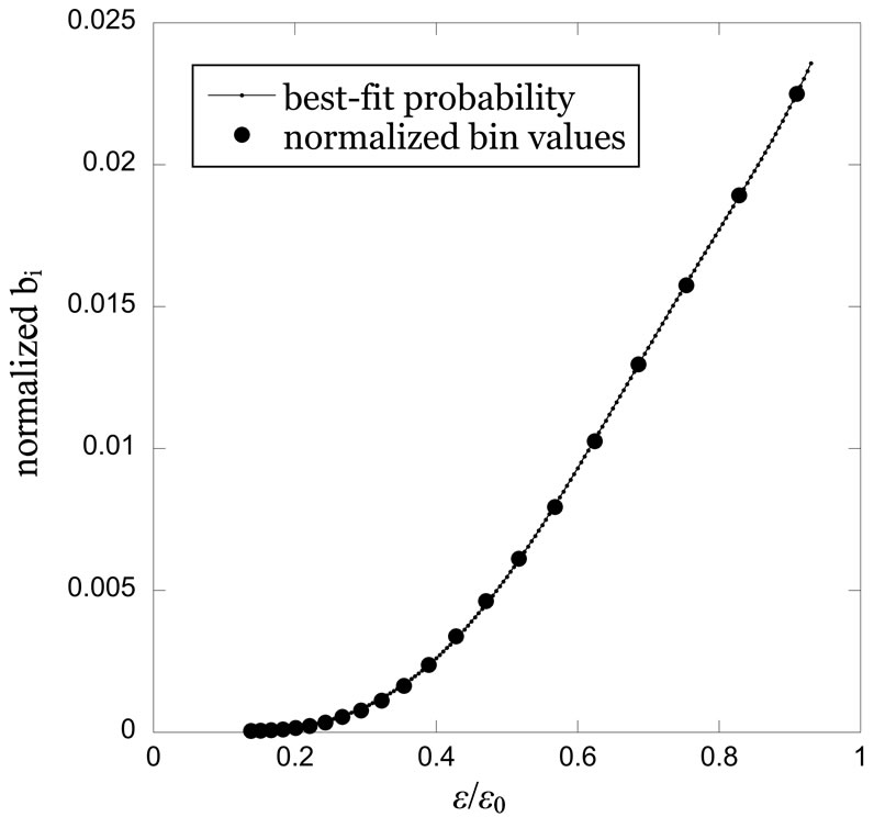
Figure 1. Normalized interpoint distance bin values for the time series based on the 20 - 40 year old age cohort data, with an embedding dimension D = 10 and cutoff value e0 = 64.2 days. Computed probabilities are based on Equation (3) using the best-fit parameters, including a correlation dimension value of d = 4.5.

Figure 2. Correlation dimension d as a function of cutoff length e0 at embedding dimensions from D = 8 to D = 12, computed from time series values based on menstrual cycle data for women aged 20 - 40 years.
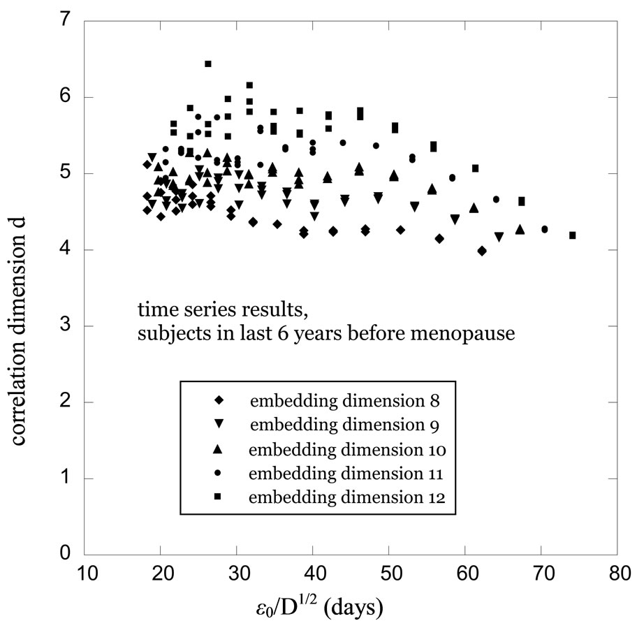
Figure 3. Correlation dimension d as a function of cutoff length e0 at embedding dimensions from D = 8 to D = 12, computed from time series values based on menstrual cycle data for women in the last 6 years before menopause.

Figure 4. Correlation dimension d as a function of cutoff length e0 at embedding dimensions from D = 8 to D = 12, computed from actual interevent time sequence values (i.e. menstrual cycles) for women aged 20 - 40 years.
results of a fitting process like that illustrated in Figure 1.
Figure 2 shows correlation dimension results, as function of cutoff value, for the analysis of a time series constructed using menstrual cycle data from women in the 20 - 40 year age range. The relatively minor variations for different embedding dimensions are depicted using differently shaped symbols. Comparable results for the correlation dimension using a time series based on menstrual cycle data from the women in the last 6 years be-

Figure 5. Correlation dimension d as a function of cutoff length e0 at embedding dimensions from D = 8 to D = 12, computed from actual interevent time sequence values (i.e. menstrual cycles) for women in the last 6 years before menopause.
fore they reached menopause are shown in Figure 3. In both of these figures the cutoff value on the horizontal axis is divided by the square root of the embedding dimension to make the results more comparable. Three major points of interest are apparent in the comparison between these two results. Firstly, the overall length scales of the two processes, indicated by the range of the cutoff values from the minimum to the maximum, are quite different in the two cases, with the characteristic length scale in Figure 3 being approximately a factor of 2 greater. Secondly, the variation of the correlation dimension with the cutoff length is significant for the 20 - 40 year old subjects, but this variation virtually nil for the subjects in the last 6 years before menopause. Thirdly, in the limit of low cutoff values, the two results for the correlation dimension become approximately equal.
Figure 4 and Figure 5 show correlation dimension results for the same subject populations as those of Figure 2 and Figure 3, respectively, but in this case we used the raw menstrual cycle data in the analysis instead of using the time series constructed from this data. Note that once again a more dramatic variation of the correlation dimension with cutoff length is observed for the 20 - 40 year old subjects than for the subjects in the last 6 years before menopause. Likewise, the characteristic length scales are roughly a factor of 2 different once again, and the limiting values of d at low e0 tend toward roughly the same values as in Figures 2 and 3. Although the d values at low e0 in Figure 4 are somewhat high compared to the others and the variations with e0 in Figure 5 are larger than those in Figure 3, these are relatively minor discrepancies given the scatter in the results. The differences between the two age cohorts that we have identified, on the other hand, are relatively large and are replicated in the two different analyses.
4. Conclusion
The important conclusion that we may infer from these results is that although the dynamics of the reproductive physiological system appear to be chaotic over the entire age range, significant changes occur in the strange attractor governing the system during the later reproductive years of the lifespan. The observed increase in the characteristic time scale involved is intuitively sensible, given the well-known increase in menstrual cycle variability during the perimenopause, but we should note that this is not merely an artifact of raw variability in the input. The standard deviations of the actual values of the fn points comprising the two different time series are approximately equal, so the difference in characteristic time scales seen in the horizontal axes of Figures 2 and 3 reflects some deeper aspect of the dynamical behavior of the system. The specific nature of these age-related changes, however, is not well understood at this time. The different behaviors of the correlation dimension with e0 are difficult to interpret without further information, and speculation about the physiological causes underlying these differences is premature at this stage. We are presently engaged in modeling the system to obtain further insight into these questions. Previous mathematical models of the menstrual cycle offer little insight, because they have assumed either periodic solutions or stochastic processes [18-20], which are inconsistent with empirical data and with the results presented here.
A potentially exciting implication of these results is that nonlinear dynamics may open new avenues to categorize and explore the lifespan development of the reproductive system. There is at present no agreement concerning even such basic issues as the definition of perimenopause or markers for when it begins [4-6]. We plan to use the methodology employed here to test some of these proposed definitions. Finally, we would suggest that these results call into question the assumption that menopause is merely the final outcome of a process of senescence, given the presence of a chaotic trajectory in both age cohorts, a presumably lawful process by which the trajectory changes, and the convergence at low e0 to similar values of the attractor’s correlation dimension in all cases.
5. Acknowledgements
We would like to thank Phyllis Mansfield and the Tremin Research Program on Women’s Health for permission to download and utilize their database of women’s menstrual histories. We would also like to thank Kevin Judd for several personal communications that clarified our understanding of his work.
REFERENCES
- H. G. Burger, G. E. Hale, L. Dennerstein, and D. M. Robertson, “Cycle and Hormone Changes during the Perimenopause: The Key Role of Ovarian Function,” Menopause, Vol. 15, No. 4, 2008, pp. 603-612. doi:10.1097/gme.0b013e318174ea4d
- P. S. Derry and G. N. Derry, “Menstruation, Perimenopause, and Chaos Theory,” Perspectives in Biology and Medicine, Vol. 55, No. 1, 2012, pp. 26-42. doi:10.1353/pbm.2012.0003
- A. Treloar, R. Boynton, B. Behn and B. Brown, “Variation of the Human Menstrual Cycle through Reproductive Life,” International Journal of Fertility, Vol. 12, No. 1, 1967, pp. 77-126.
- L. D. Lisabeth, S. D. Harlow, B. Gillespie, X. Lin and M. Sowers, “Staging Reproductive Aging: A Comparison of Proposed Bleeding Criteria for the Menopausal Transition,” Menopause, Vol. 11, No. 2, 2004, pp. 186-197. doi:10.1097/01.GME.0000082146.01218.86
- R. J. Ferrell and M. Sowers, “Longitudinal, Epidemiologic Studies of Female Reproductive Aging,” Annals of the New York Academy of Sciences, Vol. 1204, No. 1, 2010, pp. 188-197. doi:10.1111/j.1749-6632.2010.05525.x
- S. D. Harlow and P. Paramsothy, “Menstruation and the Menopausal Transition,” Obstetrics & Gynecology Clinics of North America, Vol. 38, No. 3, 2011, pp. 595-607. doi:10.1016/j.ogc.2011.05.010
- G. N. Derry and P. S. Derry, “Characterization of Chaotic Dynamics in the Human Menstrual Cycle,” Nonlinear Biomedical Physics, Vol. 4, No. 1, 2010, Article # 5. doi:10.1186/1753-4631-4-5
- J. B. Bassingthwaighte, L. S. Liebovitch and B. J. West, “Fractal Physiology,” Oxford University Press, Oxford, 1994.
- K. Prank, H. Harms, G. Brabant, R. Hesch, M. Dammig and F. Mitschke, “Nonlinear Dynamics in Pulsatile Secretion of Parathyroid Hormone in Normal Human Subjects,” Chaos, Vol. 5, No. 1, 1995, pp. 76-81. doi:10.1063/1.166089
- T. Noguchi, N. Yamada, M. Sadamatsu and N. Kato, “Evaluation of Self-similar Features in Time Series of Serum Growth Hormone and Prolactin Levels by Fractal Analysis: Effects of Delayed Sleep and Complexity of Diurnal Variation,” Journal of Biomedical Science, Vol. 5, No. 3, 1998, pp. 221-225. doi:10.1007/BF02253472
- I. Ilias, A. N. Vgontzas, A. Provata and G. Mastorakos, “Complexity and Non-linear Description of Diurnal Cortisol and Growth Hormone Secretory Patterns before and after Sleep Deprivation,” Endocrine Regulations, Vol. 36, No. 2, 2002, pp. 63-72.
- P. Mansfield and S. Bracken, “Tremin: A History of the World’s Oldest Ongoing Study of Menstruation and Women’s Health,” East Rim Publishers, Lemont, 2003.
- R. Castro and T. D. Sauer, “Forecasting and Dimension Calculations from Event Timing Data,” Nonlinear Phenomena in Complex Systems, Vol. 2, No. 3, 1999, pp. 42-51.
- F. Takens, “On the Numerical Determination of the Dimension of an Attractor,” In: B. Braaksma, H. Braer and F. Takens, Eds., Dynamical Systems and Bifurcations, Springer-Verlag, Berlin, 1985, pp. 99-106. doi:10.1007/BFb0075637
- P. Grassberger and I. Procaccia, “Characterization of Strange Attractors,” Physical Review Letters, Vol. 50, No. 5, 1983, pp. 346-349. doi:10.1103/PhysRevLett.50.346
- K. Judd, “An Improved Estimator of Dimension and Some Comments on Providing Confidence Intervals,” Physica D, Vol. 56, No. 2-3, 1992, pp. 216-228. doi:10.1016/0167-2789(92)90025-I
- K. Judd, “Estimating Dimension From Small Samples,” Physica D, Vol. 71, No. 4, 1994, pp. 421-429. doi:10.1016/0167-2789(94)90008-6
- L. H. Clark, P. M. Schlosser and J. F. Selgrade, “Multiple Stable Periodic Solutions in a Model for Hormonal Control of the Menstrual Cycle,” Bulletin of Mathematical Biology, Vol. 65, No. 1, 2003, pp. 157-173. doi:10.1006/bulm.2002.0326
- I. Reinecke and P. Deuflhard, “A Complex Mathematical Model of the Human Menstrual Cycle,” Journal of Theoretical Biology, Vol. 247, No. 2, 2007, pp. 303-330. doi:10.1016/j.jtbi.2007.03.011
- R. J. Bogumil, M. Ferin, J. Rootenberg, L. Speroff and R. L. Vande Wiele, “Mathematical Studies of the Human Menstrual Cycle. I. Formulation of a Mathematical Model,” Journal of Clinical Endocrinology & Metabolism, Vol. 35, No. 1, 1972, pp. 126-142. doi:10.1210/jcem-35-1-126
NOTES
*Corresponding author.