Journal of Power and Energy Engineering
Vol.2 No.2(2014), Article ID:43082,6 pages DOI:10.4236/jpee.2014.22003
Large Prismatic Lithium Iron Phosphate Battery Cell Model Using PSCAD
![]()
Department of Electrical and Computer Engineering, University of Massachusetts, Lowell, USA.
Email: gyessayan@gmail.com, dipesh_patel1@student.uml.edu, Ziyad_salameh@uml.edu
Copyright © 2014 Garo Yessayan et al. This is an open access article distributed under the Creative Commons Attribution License, which permits unrestricted use, distribution, and reproduction in any medium, provided the original work is properly cited. In accordance of the Creative Commons Attribution License all Copyrights © 2014 are reserved for SCIRP and the owner of the intellectual property Garo Yessayan et al. All Copyright © 2014 are guarded by law and by SCIRP as a guardian.
Received November 23rd, 2013; revised December 23rd, 2013; accepted December 31st, 2013
KEYWORDS
PSCAD; MATLAB; Curve-Fitting; Look-Up Table; Discharge Rate; Temperature
ABSTRACT
Presently, there are mainly two problems that prevent Electric Vehicles (EVs) from becoming popular against the Internal Combustion Engine Vehicles (ICEVs), namely: short range and too long to recharge the battery pack of the EV. Due to this, battery development is a crucial aspect to improve the performance of EVs. This progress requires dependable computer aided designs to model the characteristics of a battery accurately and reliably. This paper uses Power Systems Computer Aided Design (PSCAD) to create an equivalent runtime circuit model to observe the qualities of the Lithium Iron Phosphate battery cell under discharge at different temperatures. The model is a 3-R-C branch runtime equivalent circuit model. In order to find the fixed parameters of the circuit, MATLAB was used to implement basic current voltage characteristics. 3-D tables have been used in PSCAD to implement the State of Charge (SOC) and temperature dependent circuit parameters of the model. Once the simulations for all temperatures were completed, the average marginal error between measured and simulated terminal voltage came to be 2.1%, therefore making PSCAD an accurate simulation tool for modeling equivalent circuits of different batteries.
1. Introduction
One of the first battery packs used in electric vehicles was the lead acid battery. These battery packs were bulky in size, weighed close to 1000 pounds, and only provided about 16 kW/hr. Recent studies have shown that lithium based batteries provide 3 times the energy with half the weight of the lead acid batteries. The lithium based batteries are also smaller in size (100 microns thick) and deliver a higher nominal voltage (the rated voltage of the battery).
An upcoming battery that is being researched and compared to the lithium-ion battery is the lithium iron phosphate battery. The lithium iron phosphate (LiFePO4) battery ran through more than 1000 cycles before its capacity fell to 80%. This is a substantial improvement compared to the lithium-ion battery. The lithium-ion cobalt battery fell to 80% capacitance after 56 cycles [1].
More tests and comparisons were performed on both of these batteries and it was seen that by comparison with the lithium iron, phosphate battery was more suitable for electric vehicles. Some notable characteristics about the LiFePO4 battery compared to the lithium ion cobalt battery were: a lower safety risk, a higher specific energy density, being cheaper, and being more environmentally friendly.
In order to model the batteries, an accurate equivalent circuit must be constructed. There are various types of modeling methods. Some of these include physical, empirical abstract, mixed, and electrical circuit models.
The most simplistic form of modeling a battery is the the venin equivalent circuit. This circuit is shown in Figure 1. It consists of a voltage source (Voc (SOC)) that is a function of state of charge (SOC) in series with the batteries internal resistance (Rdc) and the parallel resistorcapacitor (R-C) combinations. The R-C combinations predict the response to a transient load at specific SOC’s by assuming that the open circuit voltage (Voc) is constant. Therefore, this model is unable to reflect the influence of the SOC to the battery behavior properly [2].
An impedance based circuit is shown in Figure 2. This circuit acquires an AC-equivalent impedance model in the frequency domain. It then uses a complex equivalent system (Zac) to fit the impedance ranges. This fitting process is very difficult and complex. Additionally, since these models only work for fixed SOC’s and temperatures, they cannot predict battery runtime or DC response [2].
Runtime based models, shown in Figure 3, use complex circuits to simulate the DC voltage response and runtime of the battery. This model used two different circuits to depict the battery characteristics. The circuit located to the left of Figure 3 depicts a capacitor (CQ), which contains the value of the battery capacitance, and a dependent current source which represents the batteries’ state of charge. The R-C networks, on the right side of the circuit, represent the relationship between the battery current and terminal voltage. This circuit is similar to the Thevenin’s equivalent circuit.
For this paper, a linear electrical circuit model was
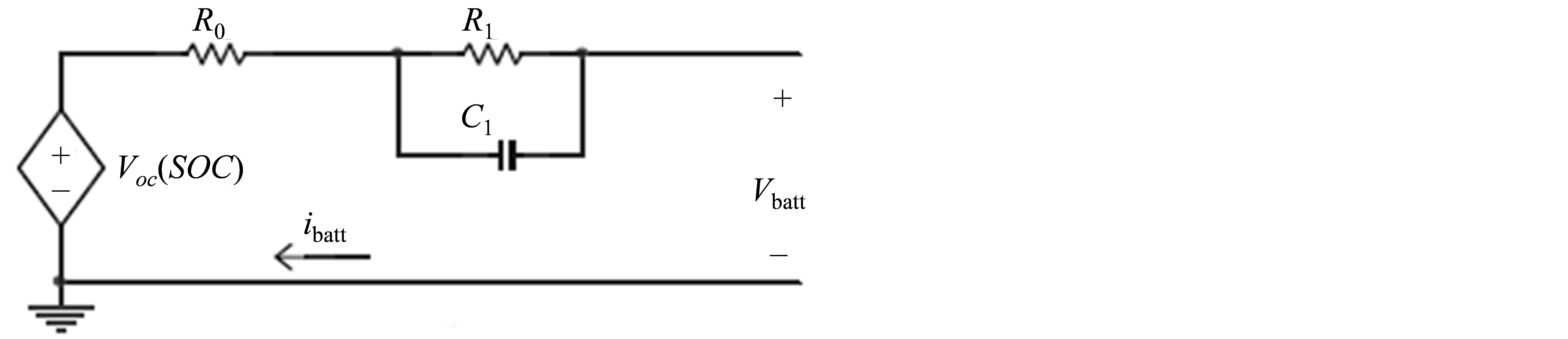
Figure 1. The Thevenin equivalent oriented battery model circuit.
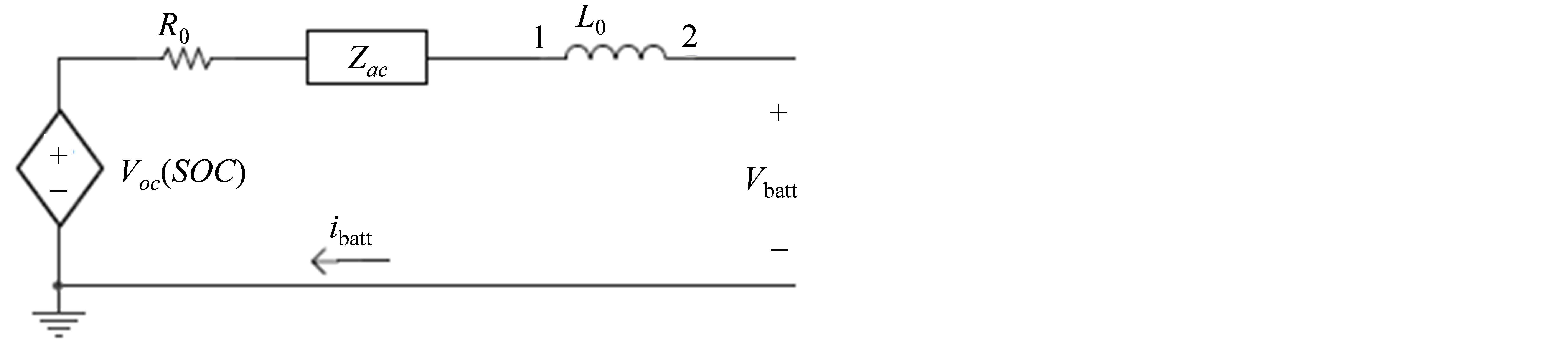
Figure 2. The impedance based oriented battery model circuit.
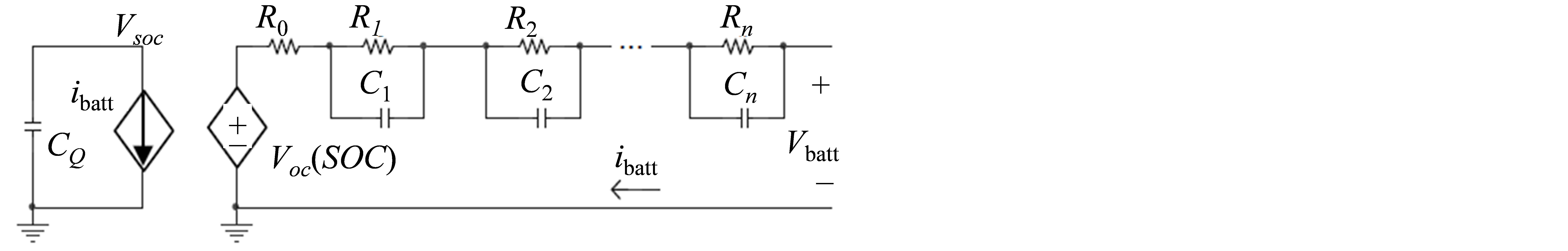
Figure 3. The runtime based oriented battery model circuit.
used based on fixed parameters given a varying state of charge (SOC). Using PSCAD, circuits were constructed using linear passive elements, voltage sources and look up tables to model the characteristics. Capacity fading was modeled using a capacitor whose capacitance decreases linearly with the number of cycles. The voltage across this capacitance represents the ratio of delivered capacity to full charge capacity. The temperature effect was modeled using a resistor-capacitor circuit with two temperature dependent sources [3].
It should be noted that this model is derived using the data gathered 6 yrs earlier, and now the batteries are completely dead due to the constant cycling and different tests. When the battery cells were tested, interval tests were not done so authors do not have the experimental data to compare it with simulation data. So model is not tested for transient behavior of the battery cell.
1.1. Battery Evaluation Lab at UMass Lowell
Since the 1990’s, there has been a battery evaluation lab at the University of Massachusetts Lowell (UML). This lab was designed to evaluate various types of batteries and their suitability for use in electric vehicles. The lab has three independent battery exerciser and data recording systems. These systems are designed to test batteries that range from 0.1 mV to 20 volts at 0.1 mA to 320 amps. Each system controls different types of current regulators that are suitable for various kinds of batteries. The batteries can be charged or discharged due to the fact that the regulators can source or sink different currents. In addition to the current regulators, there are two computer controlled environmental chambers that provide the batteries with the preferred ambient temperatures. Due to the nature of the environmental chamber, a precise analysis on the battery can be achieved to replicate the performance of the battery in an electric vehicle [4-8]. The system is shown in Figure 4.
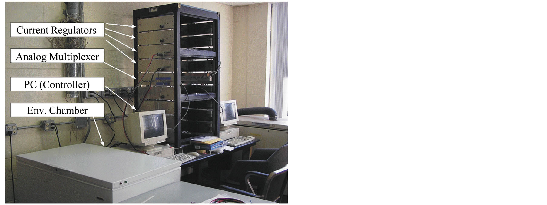
Figure 4. Battery tester at battery evaluation lab at UMass Lowell.
1.2. Battery Cell under Test to Be Modeled
This paper models the discharging battery characteristics of a lithium iron phosphate battery under various ambient temperatures (0˚C, 20˚C, 30˚C, and 40˚C). Tests are done on 160 AH lithium iron phosphate battery cells to verify the model.
2. Circuit Model
2.1. Proposed Equivalent Electrical Circuit Model
It is difficult to account for the change in battery parameters under different states of charges and conditions. Circuit based battery models use a combination of various resistors, capacitors, and voltage and current sources to model the performance of a battery. There are three basic forms of electrical models. These models include a Thevenin, Impedance model and runtime based equivalent circuit. The circuit used to evaluate this paper is the runtime based equivalent circuit [2].
For this paper a runtime based model was chosen using 3 R-C network connections. The 3 R-C networks were selected because when using 2 networks the simulation results were not matching the experimental data (error was approximately 14%). Also, the difference in plots for the experimental and measured data was negligible when using more than 3 R-C networks. Figure 5 shows the final design used to replicate the battery characteristics.
2.2. Parameter Extraction
The open circuit voltage (Voc) at each SOC was to be determined because no transient data was provided. Equation (1) was used to find Voc at each SOC.
 (1)
(1)
In Equation (1), Vt is the terminal voltage at each specific SOC (i.e. SOC = 1, SOC = 0.9, SOC = 0.8 etc.). The constant discharge current, Idis, is 80 Amps, and Rdc is the internal resistance for the respective temperature. Using the experimental data, a graph of Voc vs. SOC for each individual temperature was then plotted using MATLAB. An equation for Voc was developed by fitting the best fit curve to the graph of Voc vs SOC. Equation (2) was developed to show Voc as a function of SOC.

Figure 5. Designed circuit for battery modeling.
 (2)
(2)
where, bn is coefficients of polynomial equation of Voc
To begin finding a resistance value for the internal resistance, Rdc, the discharging data for all four temperatures was sorted out. Once the data was sorted out the nominal voltage (Vt) was found for each temperature. After finding the nominal voltage, the first voltage drop (Vd1) was obtained by using the voltage at which the current became stable. The constant discharge current (Idis) was set to 80 amps. Once all these parameters were determined, Equation (3) was used to determine Rdc.
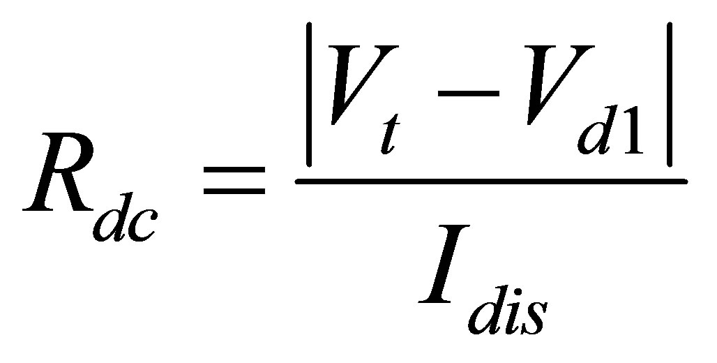 (3)
(3)
Calculation of Rdc showed that as the temperature lowers values of the Rdc increases.
In order to find R1, R2, R3, C1, C2 and C3 it is important to realize what each component does. Vd1 is the voltage after the voltage drop across internal dc resistance from open circuit voltage (Voc). Vd1 point is found using (4) and is shown in Figure 6.
 (4)
(4)
Once the Vd1 is found on voltage graph by visual inspection two other points are taken (Vd2, T2) and (Vd3, T3). These points are based on slope change criteria. As one can see the slope between (Vd1, T1) and (Vd2, T2) is steeper than the slope between (Vd2, T2) and (Vd3, T3). As the time difference between (Vd1, T1) and (Vd2, T2) is very short the R-C time constant during this period is short. The time difference between (Vd2, T2) and (Vd3, T3) is medium, the R-C time constant during this period is medium. The time difference between (Vd3, T3) and (Vd4, T4) is long, the R-C time constant during this period is long.
When looking at (5), it can be seen that the voltage Vi (branch voltage) can be considered to be the voltage drop of the low-pass filter battery current over the resistor Ri of the R-C cells [9].
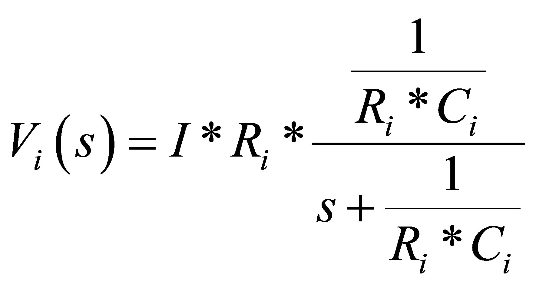 (5)
(5)
where, i is 1, 2, or 3 (1 for short time constant branch, 2 for medium time constant branch and 3 for long time constant). Ri is resistance of R-C branch. Ci is capacitance of R-C branch. I is constant current The cutoff frequency of the low-pass filter is:
 (6)
(6)
The values for Ri and Ci are calculated as a function of the SOC. Therefore, all the R’s and C’s in the R-C system cells are also calculated as functions of the SOC [9].
After finding three points as shown in Figure 6, applying (7), (8) and (9) we get R1, R2 and R3.
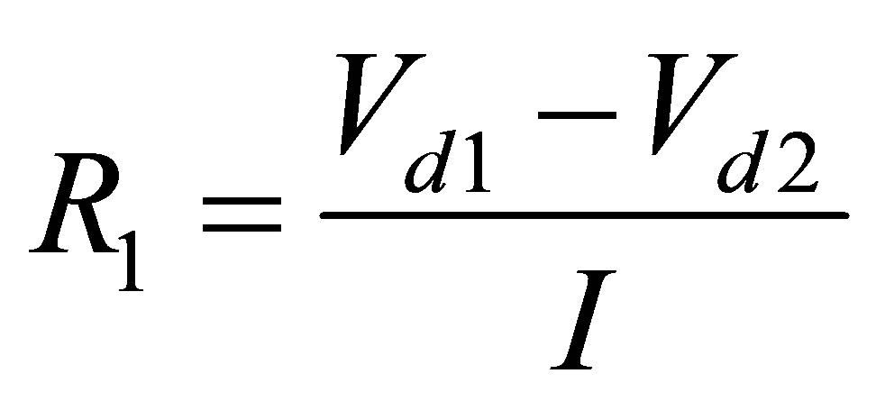 (7)
(7)
where, I is constant discharge current Given the two voltage drops and constant current, R1 was found for all ambient temperatures and discharges. R2 and R3 are found the same way as R1.
 (8)
(8)
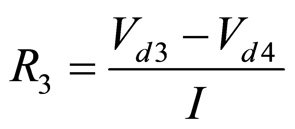 (9)
(9)
Determining the capacitance C1, C2 and C3, once R1, R2 and R3 were established, were mainly calculation based parameters. C1, C2 and C3 can be found from (10), (11) and (12),
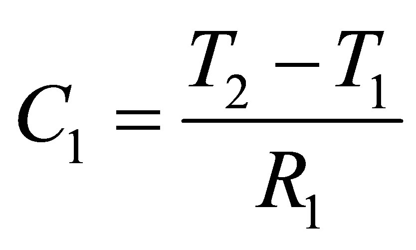 (10)
(10)
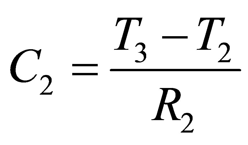 (11)
(11)
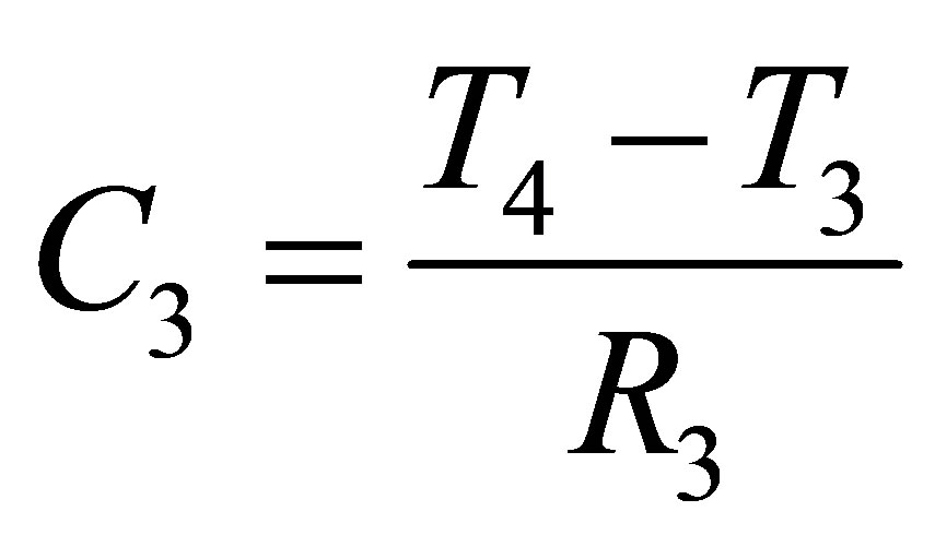 (12)
(12)
T1 is the time at which Vd1 occurs, T2 is the time at which Vd2 occurs, T3 is the time at which Vd3 occurs, and T4 is the time at which Vd4 occurs. Points Vd1, Vd2, Vd3 and Vd4 with their respective time values are shown in Figure 6.
3. PSCAD Equivalent Circuit
Once the values of all the components in the circuit (Voc, Rdc, R1, C1, R2, C2, R3, and C3) were determined it was time to simulate the circuit using PSCAD. As mentioned before, two circuits were implemented in this modeling to show constant discharge for different temperature. The first circuit consisted of a dependent current source in series with a resistor, Rs. To begin creating the circuit that is implemented into the dependent current source the following equation must be evaluated.
 (13)
(13)
In this case to ensure that the SOC was varying with time, the equation which stated that current (Ibattery) integrated from 0 to t with respect to time divided by the total battery capacitance (Cb) was substituted into PSCAD using mathematical components as shown in Figure 7.
The graphical output showed that the SOC is varying linearly over time. As mentioned before, PSCAD is mainly a mathematical modeling tool where data can be inputted into mathematical and functional components to create an equivalent model. The second circuit consists of a dependent voltage source in series with the Rdc and three parallel R-C Cells (Figure 5). PSCAD employs XYZ look up tables that were created using the data obtained from the MATLAB calculations mentioned above. XYZ look up table consists of two inputs namely SOC, and temperature or discharge rate and one output. The output can be one of the battery parameters (R1, R2, R3, C1, C2, or C3). So, the final terminal voltage depending on SOC:
 (14)
(14)
where, Rdc is equivalent dc resistance. Voc is open circuit

Figure 6. Terminal voltage vs. time.
Figure 7. Varying SOC equivalent circuit.
voltage. R1 is resistance of a short time constant parallel R-C branch. C1 is capacitance of a short time constant parallel R-C branch. R2 is resistance of a medium time constant parallel R-C branch. C2 is capacitance of a medium time constant parallel R-C branch. R3 is resistance of a long time constant parallel R-C branch. And C3 is capacitance of a long time constant parallel R-C branch.
For all the components, the X input is the temperature. Depending on the requirements X column in XYZ table can have the values for different temperatures. The Y input is the SOC, the look up table’s Z column is the calculated data. There are eight tables namely for Voc, Rdc, R1, R2, R3, C1, C2 and C3. Figure 8 shows the implementation of the second circuit, on the right of Figure 5, of the model.
Figure 9 shows the implementation of measured terminal voltage.
4. Results
Once the circuits were created in PSCAD the following simulation results were obtained. The simulation (Figure 10) of the first circuit shows the SOC of the battery with respect to the time it takes for the battery to charge. The same method can be used to simulate the discharge scenario. This model can be used to simulate the charge and discharge of the battery. The SOC in Figure 10 is shown going from 0 to 1 in approximately 7200 seconds (2 hour) based on 80 A charge of the 160 A-h lithium polymer battery. If one subtracts the value obtained as SOC in charging from 1, one gets the SOC during discharge. Initial value of the SOC is obtained by substituting the Voc value, terminal voltage just before the discharge of the battery cell commences, in (2) and solving for SOC.
After the SOC was established, it was time to simulate both the circuits, Figures 7 and 8, together. Both the terminal and simulation voltages were plotted and analyzed for each temperature. Figure 11 depicts the plot of terminal vs. simulation voltage for 0˚C.
It can be seen that the terminal and simulated plots match up fairly well. There were some discrepancies at the beginning of the graph; however those differences existed because the open circuit voltages were estimated, due to the fact that the transient data was not provided for this battery. Also, the data was recorded during long time intervals (60 seconds) which made the data less accurate than a battery that was observed over a shorter time interval (5 seconds). The maximum error for this curve was approximately 3.8%. Figure 12 portrays the plot of terminal vs. simulation voltage for 30˚C with maximum error of 1.25%.
5. Conclusion
This paper tried to successfully create an equivalent circuit in PSCAD that can model the discharge characteristics of a lithium iron phosphate battery cell at different ambient temperatures.
Due to the fact that PSCAD is only a simulator, MATLAB equations were used to determine resistor, capacitor, and open circuit voltage values. These values were then implemented into PSCAD in order to simulate how the battery operates. After completing the simulation, the results showed that PSCAD was in fact a reliable and accurate simulator for battery models. The graphs for all four temperatures matched fairly well and only had an average marginal error of approximately 2.1%. The data and graphs were also verified using MATLAB. Due to

Figure 8. Equivalent PSCAD circuit.
Figure 9. Measured terminal voltage equivalent circuit to compare it with simulated terminal voltage.

Figure 10. SOC vs. time graph.
Figure 11. Simulated and measured terminal voltage at 80 A constant discharge and at 0˚C.
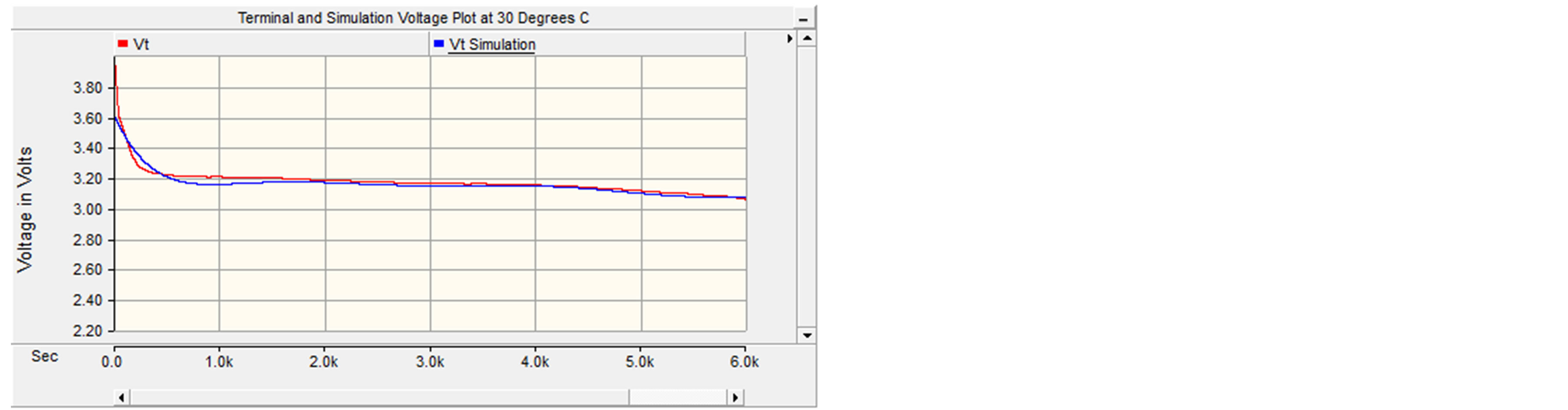
Figure 12. Simulated and measured terminal voltage vs. time at 80 A constant discharge and 30˚C.
the combination of both the same data of these softwares’ outputting, it can be concluded that PSCAD is a valid and useful tool in modeling batteries.
REFERENCES
- F. P. Tredeau, “Battery Management System,” Thesis, University of Massachusetts, Lowell, 2011.
- “Study of Battery Modeling Using Mathematical and Circuit Oriented Approaches.” http://ieeexplore.ieee.org/stamp/stamp.jsp?arnumber=06039230
- R. Ravishankar, S. Vrudhula and D. N. Rakhmatov, “Battery Modeling for Energy-Aware System Design. Battery Modeling for Energy-Aware System Design.” http://ieeexplore.ieee.org/stamp/stamp.jsp?tp=&arnumber=1250886
- F. P. Tredeau and Z. M. Salameh, “Evaluation of Lithium Iron Phosphate Batteries for Electric Vehicles Application. Evaluation of Lithium Iron Phosphate Batteries for Electric Vehicles Application.” http://ieeexplore.ieee.org/stamp/stamp.jsp?tp=&arnumber=5289704
- D. D. Patel, F. P. Tredeau and Z. M. Salameh, “Temperature Effects on Fast Charging Large Format Prismatic Lithium Iron Phosphate Cells. Temperature Effects on Fast Charging Large Format Prismatic Lithium Iron Phosphate Cells.” http://ieeexplore.ieee.org/stamp/stamp.jsp?arnumber=05729073
- Z. M. Salameh, M. A. Casacca and W. A. Lynch, “A Mathematical Model for Lead-Acid Batteries. A Mathematical Model for Lead-Acid Batteries.” http://ieeexplore.ieee.org/stamp/stamp.jsp?arnumber=00124547
- W. Lynch and Z. Salameh, “Electrical Component Model for a Nickel Cadmium Electric Vehicle Traction Battery,” Annual IEEE_PES, PP. NO, 06GM1201, Montreal, 2006. http://ieeexplore.ieee.org/stamp/stamp.jsp?arnumber=01709569
- F. Tradeau and Z. Salameh, “Characterization of the M100- 12 NiZn Battery IASTED,” Orlando, 2007.
- T. S. Hu, Z. C. Brian and J. P. Zhao, “Determining Battery Parameters by Simple Algebraic Method. Determining Battery Parameters by Simple Algebraic Method.” http://ieeexplore.ieee.org/stamp/stamp.jsp?arnumber=05990614