Received 4 April 2016; accepted 25 April 2016; published 28 April 2016

ABSTRACT

This paper describes the method of two important mathematical techniques used in chemical engineering applications. Solving a mass transfer problem, weather in finite or semi-infinite domain, may seem difficult without the practice of Finite Fourier Transform (FFT) and Similarity Transformation. Finite systems refer to any closed system that has a specific boundary that can be determined. For example, polymer sheets, membranes, storage tanks, oil reservoirs and a human stomach are determined to be finite systems where FFT is applicable to derive expressions for concentration profiles of the materials in the system. However, Similarity Transformation method is used to identify the concentration profile in semi-infinite systems that have no limits. It has been approved that we may also use the similarity procedure for finite systems since our results are almost the same. Methodologies of both techniques have been discussed thoroughly in order to apply them to a water-polymer diffusion system for the determination of the concentration of water in a polymer sheet of PET. Discussion and comparison between FFT and similarity is included to illustrate the power of each mathematical procedure in predicting and modeling mass concentrations.

Keywords:

Similarity, Fininte Fourier Transfrom, Modeling, Mass Transfer, Concentration Profile

1. Introduction

Recent advancements in applied mathematics allow engineers to encounter mass transfer problems easier than before. Emerging mathematics with engineering is necessary to solve problems in chemical engineering such as the determination of a concentration profile of material A in a binary A-B system. Difficulty of the problem depends on how many terms are; we going to deal with after applying our assumptions to the continuity equation [1] .

For instance, steady state diffusion equations are usually easy to solve compared to unsteady state or convention related problems. Additionally, considering a reaction rate will make it even harder to carry out final solution. Thus, previous established techniques including Finite Fourier Transform (FFT) and Similarity Transformation show a promising way in solving mass transfer problems and predict an approximation to the concentration profile in mass transfer systems [1] [2] . FFT is applied to finite systems while similarity is used to solve problems in a semi-infinite domain. However, similarity method is much easier than FFT and may be applied to a finite system under specific conditions [1] [3] .

Finite Fourier transform (FFT) method is one of various analytical or numerical techniques in which exact or approximate solutions to partial differential equations are found by expanding the solution in terms of a set of known functions called basis functions, and then determining the unknown coefficients in the expansion [4] .

The FFT method is fundamentally comparable to the method of separation of variables discussed in many traditional books on mathematical methods in physics and engineering; for example, see Arpaci (1966), Butkov (1968), Carslaw and Jaeger (1959), Churchill (1963), and Morse and Feshbach (1953). However, the FFT method is more flexible and easy to apply with a more direct attack on many problems. The reader who is familiar with separation of variables will easily notice the differences and the improvements suggested by the FFT method, but prior experience to separation of variables is not necessary for what is presented here [1] [4] .

The FFT is an alternative technique for solving nonhomogeneous initial boundary value problems in which time-dependent and time-independent problems are treated in exactly the same way. Also, the FFT practice can smoothly encounter and solve problems in higher dimensions. Strictly speaking, application of FFT to initial boundary value problems always follows the same pattern whether the problem is homogeneous or nonhomogeneous. The general FFT solution is always in the form of an infinite series. However, the generalized Fourier series of a simple function can show up as a part or all of the FFT solution. Thus, the FFT transform method shows its true flexibility in problems with nonhomogeneous PDEs and/or boundary conditions [2] .

The method of similarity (combination of variables) is useful for semi-infinite systems, such that the initial condition and the boundary condition at infinity may be combined into a single new boundary condition [1] . The similarity technique reduces a partial differential equation in two independent variables to an ordinary differential equation involving a single composite variable. Similarity analysis is applicable to certain problems in which the characteristic lengths are determined by rate processes, rather than by the geometric dimensions. In particular, the technique is applied to problems that generally involve regions which are regarded as being semi-infinite. The method may be used with linear and nonlinear problems [4] .

In this work, we would like to show the methodology of each technique and solve one common problem to identify the differences between both methods. A discussion section is included to confirm our results, understand the physical meaning of the equations and compare between both results for further purposes.

2. Finite Fourier Transform

2.1. Methodology

1) Write the governing equation, initial and boundary conditions after applying the given assumptions.

2) Make the governing equation in a dimensionless form.

3) Write the initial and boundary conditions in dimensionless forms.

4) Define a new eigenvalue problem () from the dimensionless governing equation in Step (2) to get the transient solution (); then solve for () by using FFT in Table 1 depending on the boundary conditions.

5) Continue solving for the transient solution () by multiplying the dimensionless governing equation in

Step (2) by the solution () we get in Step (4) and take the integration for all terms. Note that we

take the integration with respect to the variable that we solved for in the eigenvalue problem () and here we have () because we solved for in our example.

6) Solve each integration independently; then, put everything back into the dimensionless governing equation in Step (2) and solve it analytically if possible.

^*δ = Length or thickness, z = coordinate axis.

7) Write down the final transient solution ().

8) Now, solve for the steady state solution (); where; change in time is zero since.

9) Apply the formula to find the overall unsteady state solution.

10) Apply the dimensionless initial condition from Step (3) and the orthogonality property into Step (9) overall unsteady state solution and solve for the constant. You can solve for the constant by multiplying

all terms by the same function that remained in the summation and, then, take the integration for all terms and apply orthogonality.

11) Substitute the constant back into Step (9) and rewrite the overall specific solution of the unsteady state problem.

2.2. An Example in Diffusion of Water in a Polymer

Assume that we have a polyethylene terephthalate (PET) tile that is stored for a time before extruding. PET will absorb moist (water) from the air and may plug the extruder when being processed. Therefore, we are interested in studying the concentration of water in the PET sheet. Solution to this problem is important because we need to determine how much water is diffused into the PET with respect to time and space [1] [5] . Obviously, our system is finite and we can solve the problem by applying FFT method. We have a binary system of A and B in which we are studying the mass transfer of component A (water) into component B (PET). Figure 1 shows a schematic to the problem with PET boundaries and assuming that there is diffusion from the topside only since the tile is very thin.

Step (1):

Let us start the solution by using the continuity equation in Cartesian coordinates since the PET tile is a plane system [1] [6] .

(1)

where; is the concentration of water in the PET tile, is diffusivity of A (water) into B (PET), is the reaction rate of A, is the velocity of component A in the x coordinate, t is the time and are the Cartesian coordinates of the system.

Assumptions:

a) Mass transfer occurs by diffusion only (no convention).

b) Mass transfer is only in the z-direction.

c) No reaction.

Thus, Equation (1) becomes:

(2)

Initial condition (I.C.):

(3)

Boundary conditions (B.C.’s):

(4)

Step (2):

Let to be the dimensional concentration of component A (water) [1] [6] :

(5)

is the initial concentration of the water in the PET at. Make everything dimensionless and convert space and time into a dimensional form as follows [1] [6] :

(6)

where; refers to the PET tile thickness. The governing equation in Equation (2) becomes:

(7)

Step (3):

Dimensionless I.C.:

(8)

Dimensionless B.C’s.:

(9)

We can write the dimensionless B.C.’s as follows:

(10)

Step (4):

Define a new eigenvalue problem by selecting the term with the higher derivative order in Equation (7).

(11)

where; is a constant and is the defined eigenvalue function. Solving for gives:

(12)

Applying dimensionless B.C.’s from Equation (9), Equation (10) or by using Table 1 at, we get:

(13)

where; n refers to the summation number and in the range; is defined from FFT as follows:

(14)

Step (5):

Solving for the transient solution (); multiply the dimensionless governing equation in Equation (7) by

and integrate, this yield to:

(15)

Step (6):

Solve the integration of each part in Equation (15) independently.

(16)

(17)

(18)

(19)

(20)

(21)

Also, from Table 1 and since we used the B.C.’s at from Equation (10) to determine the solution; we must have, (Case II), therefore:

(22)

(23)

Plug Equations (21), (22) and (23) into Equation (17), then plug Equations (16) and (17) into Equation (15).

(24)

Equation (24) is a separable differential equation which can be solved easily to get [7] - [9] :

(25)

Apply I.C. from Equation (8) to get, hence:

(26)

Step (7):

The final transient solution is

(27)

(28)

Step (8):

Solve for the steady state solution

(29)

Thus, Equation (7) becomes:

(30)

Apply B.C. from Equation (9),

(31)

(32)

Step (9):

The overall solution is

(33)

(34)

Step (10):

Applying I.C. from Equation (8) and orthogonality to get the constant [7] [8] .

(35)

Multiply both sides by and integrate

(36)

(37)

(38)

Step (11):

Plug Equation (38) and Equation (14) into Equation (34), the overall specific solution is as follows:

(39)

Let us assume our dimensional space to be in this notation () to compare with the similarity example.

(40)

where;

(41)

At steady state: ()

(42)

3. Similarity Transformation

3.1. Methodology

1) Write the governing equation, initial and boundary conditions after applying the given assumptions.

2) Make the governing equation in a dimensionless form.

3) Write the initial and boundary conditions in dimensionless forms.

4) Propose a dimensionless combinations solution that will satisfy our problem. However, the proposed solution is usually in form of.

5) Apply the chain rule to each derivative term in the dimensionless governing equation in Step (2). Use our proposed solution () in step 4 to carry out the chain rule derivatives.

6) Substitute the new relations that you get back into the dimensionless governing equation in Step (2).

7) Solve the dimensionless governing equation and get the general solution.

8) Apply the dimensionless boundary conditions from Step (3) to find constants, hereafter the specific solution.

3.2. An Example in Diffusion of Water in a Polymer

Here, we need to solve the same previous problem (FFT) with the Similarity transformation procedure. The only parameter that will change is the boundary conditions since we are dealing with semi-infinite domain in this method. In other words, the PET polymer sheet is considered as a semi-infinite system that has no boundaries from one side which makes. Figure 2 shows a schematic to the problem with the PET boundaries in Similarity method.

Step (1):

We can start our solution from Equation (2) since we have the same assumptions.

(43)

I.C.:

(44)

B.C.’s: assume

(45)

Step (2):

Dimensionless concentration, time and space [1] [6] :

(46)

(47)

Plug Equations (46) and (47) into Equation (43) to get the dimensionless governing equation:

(48)

Step (3):

Dimensionless I.C.:

(49)

Dimensionless B.C.’s:

(50)

Step (4):

where;

(51)

Step (5):

Use Equation (51) to apply the chain rule to Equation (48) with respect to

(52)

(53)

(54)

Step (6):

Plug Equation (52) and (54) into Equation (48) to get:

(55)

(56)

Step (7):

Solution to Equation (56) gives:

(57)

Step (8):

Apply dimensionless B.C.’s from Equation (50) to determine the constants

(58)

(59)

Thus, final specific unsteady state solution becomes:

(60)

(61)

At steady state:

(62)

4. Results and Discussions

Comparing both results obtained from FFT strategy and Similarity transformation will allow us to analyze the credibility of each method. We wish to study the differences in both steady state and unsteady state systems. By comparing the steady state solution from Equation (42) and Equation (62), we realize that FFT and Similarity transformation gave the same result. However, we want to see weather changing the domain of a problem from its finite domain to a semi-infinite system in the unsteady state situation will have an impact on our results or not. Equalizing similar terms in both solutions would allow us to find an estimation for the diffusivity. We have confirmed our solutions in different ways to ensure that we have correct answers in both methods.

Combining Equation (40) and Equation (61) gives:

(63)

Take the derivative with respect to (z) for both sides in Equation (63); and consider only the first term in the summation at; neglect other terms since they will have smaller values.

(64)

(65)

Thus, if diffusivity value is not constant, we can estimate the diffusivity at any time and space within the system from Equation (65). We know that the general solution for the unsteady state diffusion equation is [10] :

(66)

where; b is a constant and must be and is an imaginary unit. Equation (66) is the general complex solution to the diffusion Equation (7); and their real and imaginary parts are both solutions [10] .

(67)

(68)

Our FFT solution in Equation (40) is identical to the general diffusion solution formula in Equation (68). Therefore, FFT complex solution must be correct. Comparison of both Equations gives:

(69)

Now, we need to confirm the Similarity transformation solution from the concentration profile plot. Data is assumed as shown in Table 2, and then applied in Equation (61).

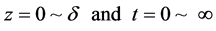
Figure 3 showed that Similarity solution to our problem is logical. Dimensionless concentration is at the maximum at the PET surface where the water concentration at this place is at its peak value since it is at the interface between moist air and PET tile [5] . On the other hand, dimensionless concentration is close to zero and at its minimum value at the end of the tile thickness. Concentration is decreasing linearly as thickness becomes larger since the water diffusion becomes weaker at the inside areas. Moreover, the higher the exposure diffusion time we have the more water concentration we notice in the PET. Figure 4 shows that higher exposure times such as one day or two will result in having a minimum concentration at the PET thickness that is more than one half of the initial concentration that is at the membrane surface. Similarity solution explained the concentration profile perfectly which making Similarity transformation technique is a viable option in finite systems as well as the semi-infinite domains.

5. Conclusion

Solutions to the given example show identical results in both steady and unsteady state systems for finite and

^*Diffusivity is calculated at 32˚C from:; [11] .

semi-infinite domains. Although similarity is mostly used in semi-infinite systems, it may also be used to determine approximated results for finite systems such as diffusion of water into a polymer; specifically the diffusion of moist air into the PET tile. Confirmation to our solutions is initiated by different mathematical manipulations. FFT solution is approved by comparing the final solution with the general solution formula for the diffusion equation. However, confirmation of similarity procedure is achieved by substituting assumed data and plotting the results which predict that we have a logical answer.

Acknowledgements

The author would like to acknowledge the Saudi Arabian Cultural Mission (SACM) for their continuous support, fund and encouragement to accomplish this work.

Cite this paper

Hisham A. Maddah,1 1, (2016) Application of Finite Fourier Transform and Similarity Approach in a Binary System of the Diffusion of Water in a Polymer. Journal of Materials Science and Chemical Engineering,04,20-30. doi: 10.4236/msce.2016.44003

References

- 1. Bird, R.B., Stewart, W.E. and Lightfoot, E.N. (2002) Transport Phenomena. 2nd Edition, John Wiley & Sons Ltd., New York.
http://dx.doi.org/10.1115/1.1424298 - 2. Trim, D.W. (1990) Applied Partial Differential Equations. 1st Edition, Pws Pub Co., Boston.
- 3. Welty, J., Wicks, C.E., Wilson, R.E. and Rorrer, G.L. (2007) Fundamentals of Momentum, Heat, and Mass Transfer. 5th Edition, John Wiley & Sons Ltd., New York.
- 4. Deen, W.M. (2011) Analysis of Transport Phenomena. 2nd Edition, Oxford University Press, New York.
- 5. Ramachandran, P.A. (2014) Advanced Transport Phenomena: Analysis, Modeling, and Computations. 1st Edition, Cambridge University Press, New York.
- 6. Bergman, T.L., Lavine, A.S., Incropera, F.P. and DeWitt D.P. (2011) Fundamentals of Heat and Mass Transfer. 7th Edition, John Wiley & Sons Ltd., New York.
- 7. Greenberg, M.D. (1998) Advanced Engineering Mathematics. 2nd Edition, Prentice Hall, New Delhi.
- 8. Kreyszig, E. (2011) Advanced Engineering Mathematics. 10th Edition, John Wiley & Sons Ltd., New Delhi.
- 9. Myint-U, T. and Debnath, L. (2006) Linear Partial Differential Equations for Scientists and Engineers. 4th Edition, Birkhäuser, Boston.
- 10. Cushman-Roisin, B. (2012) Environmental Transport and Fate. 1st Edition, Dartmouth College, USA.
- 11. Green, D.W. and Perry, R.H. (2007) Perry’s Chemical Engineers’ Handbook. 8th Edition, McGraw-Hill Professional, New York.