Journal of Applied Mathematics and Physics
Vol.04 No.07(2016), Article ID:67936,10 pages
10.4236/jamp.2016.47124
An Analytical Model for Multifractal Systems
Jun Li
Key Laboratory of Mountain Surface Process and Hazards/Institute of Mountain Hazards and Environment, Chinese Academy of Sciences, Chengdu, China
![]()
Copyright © 2016 by author and Scientific Research Publishing Inc.
This work is licensed under the Creative Commons Attribution International License (CC BY).
http://creativecommons.org/licenses/by/4.0/


Received 7 June 2016; accepted 1 July 2016; published 4 July 2016
ABSTRACT
Previous multifractal spectrum theories can only reflect that an object is multifractal and few explicit expressions of f(α) can be obtained for the practical application of nonlinearity measure. In this paper, an analytical model for multifractal systems is developed by combining and improving the Jake model, Tyler fractal model and Gompertz curve, which allows one to obtain explicit expressions of a multifractal spectrum. The results show that the model can deal with many classical multifractal examples well, such as soil particle-size distributions, non-standard Sierpinski carpet and three-piece-fractal market price oscillations. Applied to the soil physics, the model can effectively predict the cumulative mass of particles across the entire range of soil textural classes.
Keywords:
Multifractal, Jake-Jun Model, Cantor Set, Sierpinski Carpet, Price Oscillation

1. Introduction
A multifractal system is a generalization of a fractal system in which a single exponent (the fractal dimension) is not enough to describe its dynamics; instead, a continuous spectrum of exponents is needed [1] . Two main mathematical languages of multifractal spectrum were proposed to estimate the multifractal systems. One is the graph of Dq vs. q [2] - [4] , where Dq is the generalized dimension for a dataset and q is an arbitrary set of exponents. Another useful multifractal spectrum is the graph of f(α) vs. α [5] , where f(α) is the Hausdorff dimension and α is the singularity strength. The f(α) and Dq can be linked together by the Legendre transformation.
However, the direct determination of a statistically stable and accurate f(α) from real world data is often considered problematic because it demands large amounts of data samples, besides being susceptible to large errors due to logarithmic corrections [6] - [8] . At the same time, when the multifractal spectrum is estimated using the “box-counting” method and the “sand box” method [9] [10] , much more numerical computation is required. Moreover, these theory techniques expressed the multifractal analysis results in terms of the measure’s multifractal spectrum, Dq vs. q or f(α) vs. α, which are only the graphs and do not yield explicit expressions for the functions describing the behavior of a multifractal system [11] . The multifractal spectrum curves can only reflect that an object is multifractal, and fail to solve the crucial problem: How can this nonlinearity measure be used [12] ? For example, the multifractal spectrum graph of a soil particle-size distribution (PSD) reflects detailed multifractal information of soil PSD [13] [14] , but the multifractal spectrum graph does not yield explicit expressions that cannot be used to effectively predict soil hydraulic properties in soil hydrology and soil physics investigations.
In this paper, an analytical model for multifractal systems is developed by combining and improving the Jaky model, Tyler fractal model and Gompertz curve, which allows one to obtain explicit expressions of a multifractal spectrum.
2. Description of Methods
2.1. Theory of Jake-Jun Model
Jaky [15] proposed the following model to characterize grain-size distribution in sediments:
 . (1)
. (1)
where F2 is the cumulative mass of particles with equivalent diameter ≤ d (mm); p is the index characterizing the stretching of the curve; and d0 is the largest diameter (mm).
The Jake model produces a sigmoidal shape similar to the left-hand side of a Gaussian lognormal distribution. This model was first introduced into the soil science literature from the geotechnical discipline by Buchan et al. [16] . The study of Buchan showed that the Jake model provided a good fit to data for many of the soils examined, and was better than the standard lognormal model [17] . Hwang and Powers found that the Jake model for generating PSD input, resulted in the best estimate for soil hydraulic properties of most soils that they examined [18] .
Mandelbrot first established the fractal PSD model for two-dimensional space [19] :
 . (2)
. (2)
where A(r > R) is the cumulative mass of grain sizes “r” larger than a specific measuring scale R; Ca and λa are constants relating to the shape factors and total range of scale; and D is the fractal dimension. Tyler and Wheat craft established the fractal PSD model for three-dimensional space based on Mandelbrot’s study [20] :
 . (3)
. (3)
where MT is the total mass of particles and D is the fractal dimension for particles. In order to compare Equation (1) and Equation (3), they are standardized as:
 (4)
(4)
![]() . (5)
. (5)
Figure 1 shows the curves of F1 and F2 distributed on the USDA textural triangle. The red solid lines repre- sent the loci of soils whose mass distribution follows Equation (4) and Equation (5) exactly. However, well- graded soils, such as a silty loam, are not well described by Equation (4) and Equation (5) since they do not fall near the red lines. Thus, it is clear that soil texture affects the performance of the one-parameter model. Given these restrictions for some soil textures, it becomes apparent that difficulties may arise in using the one-para- meter model as the input for quantitative simulation of soil structure and hydraulic properties.
The expression forms of Equation (4) and Equation (5) are very similar, differing only in their exponent. This provides a very useful insight that if the exponent is set to a variable parameter, we can enhance the Jake PSD model to cover all the soil textural classes. The enhanced Jake model (named “Jake-Jun” model based on two researchers’ name: the author of the Jake Model, “Jake”, and the author of this paper, “Jun”, for convenience) proposed by this study has two parameters and is expressed as:
![]() . (6)
. (6)
![]()
Figure 1. The curves of F1 and F2 distributed to the USDA textural triangle {F1, D = [0, 3]); F2, p = (0, +∞)}.
where F(r ≤ d) is the cumulative mass of particles with equivalent diameter ≤ d; d0 is the largest diameter; m is an exponential factor that is the extension of the Jake model exponential form; and D is the fragmentation fractal dimension incorporated from the Tyler fractal model. The Jake-Jun model can be utilized for the entire textural triangle for predicting the cumulative mass of particles across the entire range of soil textural classes (Figure 2).
For Equation (6), we assume that the complex fractal (m > 1) derived from natural evolution of simple fractals (m = 1) remains unchanged in fractal dimension D during soil developmental evolution, then
![]() ,
,![]() . (7)
. (7)
To introduce a time variable t, we set
![]() ,
, ![]() , (8)
, (8)
which corresponds to
![]() ,
,![]() . (9)
. (9)
Equation (7) is the well-known Gompertz curve. A Gompertz curve, named after Benjamin Gompertz, is a sigmoid function, such as a growth curve. It is a type of mathematical model for a time series, where growth is slowest at the start and end of a period.
2.2. Jake-Jun Model and Lognormal Distribution
The lognormal cascade model that the probability density function of data set successive increments at different time scales was introduced to study of fully developed turbulence [21] [22] . Burlaga [23] found that the multifractal spectrum of the magnetic field strength fluctuations could be described by the symmetric function given by the multiplicative cascade model [24] . These studies showed that the lognormal distribution closely related to multifractal systems. The most common lognormal distribution given by:
![]() (10)
(10)

Figure 2. The contour of m distributed to the USDA textural triangle {F, m = (0, 10]}.
The cumulative distribution of lognormal distribution function is
 . (11)
Jake-Jun model is the cumulative mass distribution function of particles. We can get its probability density function (particle mass of x layer) by first derivative of F(x):
 . (12)
When m = 2, comparing Equation (10) and Equation (12), to set
 ,
, . (13)
Equation (12) can be normalized to
 . (14)
From this, Jake-Jun model is the variations and combinations of a lognormal distribution function. This expansion have two aspects: one the hand, the exponent “2” in a lognormal distribution function becomes the variable parameter m; On the other hand, the amplitude is combined with a logarithm function. To understand parameters m and D, we produced their contour maps (Figure 3 and Figure 4). They show that Jake-Jun model may describe single-peak skewed distribution events.
2.3. Multifractal Spectrum of Jake-Jun Mode
A mass distribution may be spread over a region in such a way that the concentration of mass is highly irregular. There are two basic approaches to multifractal analysis: fine theory, where we examine the structure and dimensions of the fractals that arise themselves, and coarse theory, where we consider the irregularities of distribution of the measure of balls of small but positive radius r and then take a limit as r → 0 [25] .

Figure 3. The contour of m distributed {G(x), D = 0.291, m = (0.75, 3)}.

Figure 4. The contour of D distributed {G(x), m = 2.51, D = (2.91, 2.98)}.
Compared to a unifractal, a multifractal can be understood as the more general relationships that the dimension of a unifractal is also a function of the scale of observation. In the Jake-Jun model, we set:
 . (15)
With Equation (6), we get
 . (16)
Equation (16) is the explicit expression of multifractal dimension in Jake-Jun model. When m = 1, Dk = D is the Hausdorff dimension of a unifractal. To set k = 2−n, Figure 5 shows the multifractal spectrum that is a map for Dk and ln (1/k) with a series values of m.
Jake-Jun model thinks of a multifractal as the variation of a unifractal. Its basis is a unifractal with Hausdorff dimension D and it uses the variation parameter m to simulate a multifractal. Therefore, the explicit expression (Equation (16)) of multifractal spectrum has parameters D, m and observation scale k.
2.4. Jake-Jun Model and f(α)
The Jake-Jun model isn’t just a PSD model, but a new multifractal system. In the multifractal spectrum of f(α) vs. α, the respective measure of the ith cell at every size scale ε is defined by mi = εα and the number of cells N(mi) with singularity strength falling within α given α and α + dα is considered as  [5] . In fact, Jake-Jun model have simulated the cumulative mass distribution function of mi. Let

Figure 5. The multifractal spectrum of Jake-Jun mo- del (set k = 2−n).
 ,
,  ,
,  ,
, . (17)
The cumulative mass distribution function of mi is:
 . (18)
When Equation (18) is regarded a continuous function, such that
 . (19)
According to Equation (12) and Equation (19), we have
 . (20)
Therefore, the explicit expressions of f(α) using Jake-Jun model is
 . (21)
where
 ,
,  ,
, .
.
When Equation (18) is regarded a discrete function, such that
 (22)
(22)
 . (23)
3. Application to Multifractal Systems
3.1. Non-Standard Sierpinski Carpet
The Sierpinski carpet (Figure 6(a)) is a generalization of the Cantor set to two dimensions. In order to display visually the multifractal principle of Jake-Jun model using the fractal idea of Sierpinski carpet, we remove the sub squares in non-standard places, such as Figure 6(b).
The construction of the Sierpinski carpet begins with a square which length is L. The square is cut into b2 congruent sub squares in a b-by-b grid, and K sub squares are removed. The same procedure is then applied recursively to the remaining C sub squares, ad infinitum. In standard Sierpinski carpet, the same K is used for each iteration and it is a single fractal. Set ,
,  ,
,  ,
, .
.
When m = 1 in Equation (6), it is a unifractal, then
 . (24)
If we use different K for iteration and then it will be a multifractal Sierpinski carpet. We set
 . (25)
Using Equation (6), we get:
 . (26)
Given the parameters D and m, Cn and can be calculated:
 . (27)
 . (28)
Therefore, the multifractal mechanics of Jake-Jun model can be visualized demonstration using the Sierpinski carpet (Figure 7).
3.2. Three-Piece-Fractal Generator
Mandelbrot [26] thinks that variations in financial prices can be accounted for by a model derived from multifractal. They do create a more realistic picture of market risks. He used the Three-piece-fractal generator (Figure 8) to simulate market price oscillations.
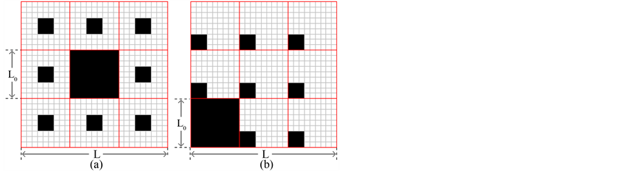
Figure 6. (a) Standard Sierpinski carpet; (b) non-standard Sierpinski carpet.
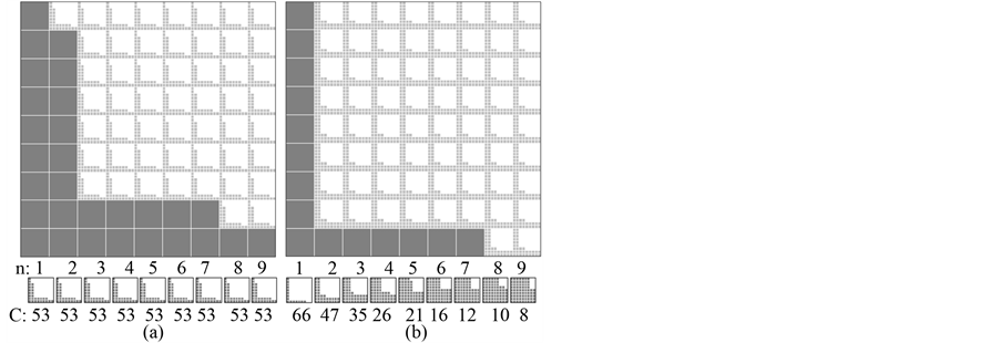
Figure 7. Non-standard Sierpinski carpets with the single fractal and the multifractal. (a) is a single fractal (D = 1.807; F(r ≤ Rn) = 53n/92n). (b) is a multifractal (D = 1.807, m = 1.85518; F(r ≤ Rn) = C1C2C3 … Cn/92n), where Cn are calculated from Equation (6).
Three-piece-fractal generator can be interpolated repeatedly into each piece of subsequent charts. The pattern that emerges increasingly resembles market price oscillations (Figure 9).
Mandelbrot’s Three-piece-fractal is that these self-affine fractal curves exhibit a wealth of structure―a foundation of both fractal geometry and the theory of chaos. However, Mandelbrot did not give a quantitative description of these self-affine fractal curves. The surprise is that Jake-Jun model can finish the task. If we think these segments of the Three-piece-fractal multifractal as particles (Figure 9) and the height (price) as the parameter d, we find that Jake-Jun model can simulate this multifractal very well. Figure 10 shows the simulation results which correlation coefficients are greater than 0.99.

Figure 8. Three-piece-fractal generator [26] .
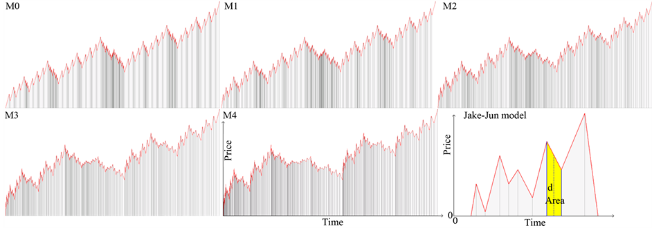
Figure 9. Three-piece-fractal generator can be interpolated repeatedly into each piece of subsequent charts. The pattern that emerges increasingly resembles market price oscillations.
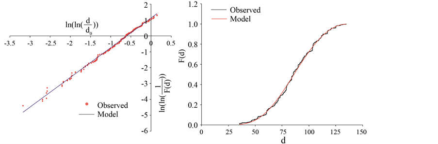
Figure 10. The simulation results of Three-piece-fractal multifractal using Jake-Jun model.
4. Conclusion
In conclusion, an analytical model (named Jake-Jun model) for multifractal systems was developed by combining and improving the Jake model, Tyler fractal model and Gompertz curve. Previous multifractal theories fail to solve the crucial problem, “How can this nonlinearity measure be used?”, because few explicit expressions of f(α) can be obtained. The Jake-Jun model has solved the crucial problem using the mass cumulative distribution function. The Jake-Jun model is able to deal with many classical multifractal examples well, such as soil particle-size distributions, two-scale Cantor set, non-standard Sierpinski carpet and three-piece-fractal market price oscillations. It is an accurate and simple approach for modeling multifractal systems from experimental data. The Jake-Jun model would be able to apply in soil hydraulic, rainfall distribution, basin structure and in many other multifractal systems.
Cite this paper
Jun Li, (2016) An Analytical Model for Multifractal Systems. Journal of Applied Mathematics and Physics,04,1192-1201. doi: 10.4236/jamp.2016.47124
References
- 1. Harte, D. (2001) Multifractals: Theory and Applications. CRC Press, Boca Raton.
http://dx.doi.org/10.1201/9781420036008 - 2. Hentschel, H.G.E. and Procaccia, I. (1983) The Infinite Number of Generalized Dimensions of Fractals and Strange Attractors. Physica D: Nonlinear Phenomena, 8, 435-444.
http://dx.doi.org/10.1016/0167-2789(83)90235-X - 3. Grassberger, P. (1983) On the Fractal Dimension of the Henon Attractor. Physics Letters A, 97, 224-226.
http://dx.doi.org/10.1016/0375-9601(83)90752-1 - 4. Grassberger, P. and Procaccia, I. (1984) Dimensions and Entropies of Strange Attractors from a Fluctuating Dynamics Approach. Physica D: Nonlinear Phenomena, 13, 34-54.
http://dx.doi.org/10.1016/0167-2789(84)90269-0 - 5. Halsey, T.C., Jensen, M.H., Kadanoff, L.P., Procaccia, I. and Shraiman, B.I. (1986) Fractal Measures and Their Singularities: The Characterization of Strange Sets. Physical Review A, 33, 1141.
http://dx.doi.org/10.1103/PhysRevA.33.1141 - 6. Chhabra, A. and Jensen, R.V. (1989) Direct Determination of the f(α) Singularity Spectrum. Physical Review Letters, 62, 1327-1330.
http://dx.doi.org/10.1103/PhysRevLett.62.1327 - 7. Arneodo, A., Bacry, E. and Muzy, J.F. (1995) The Thermodynamics of Fractals Revisited with Wavelets. Physica A: Statistical Mechanics and Its Applications, 213, 232-275.
http://dx.doi.org/10.1016/0378-4371(94)00163-N - 8. Welter, G.S. and Esquef, P.A. (2013) Multifractal Analysis Based on Amplitude Extrema of Intrinsic Mode Functions. Physical Review E, 87, Article ID: 032916.
http://dx.doi.org/10.1103/physreve.87.032916 - 9. Tél, T., Fülöp, á. and Vicsek, T. (1989) Determination of Fractal Dimensions for Geometrical Multifractals. Physica A: Statistical Mechanics and Its Applications, 159, 155-166.
http://dx.doi.org/10.1016/0378-4371(89)90563-3 - 10. Vicsek, T. (1990) Mass Multifractals. Physica A: Statistical Mechanics and Its Applications, 168, 490-497.
http://dx.doi.org/10.1016/0378-4371(90)90401-D - 11. Olsen, L. (2013) Multifractal Tubes. In: Barral, J. and Seuret, S., Eds., Further Developments in Fractals and Related Fields, Birkhäuser, Boston, 161-191.
http://dx.doi.org/10.1007/978-0-8176-8400-6_9 - 12. Ausloos, M. (2012) Measuring Complexity with Multifractals in Texts. Translation Effects. Chaos, Solitons and Fractals, 45, 1349-1357.
http://dx.doi.org/10.1016/j.chaos.2012.06.016 - 13. Grout, H., Tarquis, A.M. and Wiesner, M.R. (1998) Multifractal Analysis of Particle Size Distributions in Soil. Environmental Science and Technology, 32, 1176-1182.
http://dx.doi.org/10.1021/es9704343 - 14. Posadas, A.N., Giménez, D., Bittelli, M., Vaz, C.M. and Flury, M. (2001) Multifractal Characterization of Soil Particle-Size Distributions. Soil Science Society of America Journal, 65, 1361-1367.
http://dx.doi.org/10.2136/sssaj2001.6551361x - 15. Jaky, J. (1944) Soil Mechanics. Egyetemi Nyomda, Buhdapest. (In Hungarian)
- 16. Buchan, G.D., Grewal, K.S. and Robson, A.B. (1993) Improved Models of Particle-Size Distribution: An Illustration of Model Comparison Techniques. Soil Science Society of America Journal, 57, 901-908.
http://dx.doi.org/10.2136/sssaj1993.03615995005700040004x - 17. Buchan, G.D. (1989) Applicability of the Simple Lognormal Model to Particle-Size Distribution in Soils. Soil Science, 147, 155-161.
http://dx.doi.org/10.1097/00010694-198903000-00001 - 18. Hwang, S.I. and Powers, S.E. (2003) Using Particle-Size Distribution Models to Estimate Soil Hydraulic Properties. Soil Science Society of America Journal, 67, 1103-1112.
http://dx.doi.org/10.2136/sssaj2003.1103 - 19. Mandelbrot, B.B. (1983) The Fractal Geometry of Nature. American Journal of Physics, 51, 286.
http://dx.doi.org/10.1119/1.13295 - 20. Tyler, S.W. and Wheatcraft, S.W. (1992) Fractal Scaling of Soil Particle-Size Distributions: Analysis and Limitations. Soil Science Society of America Journal, 56, 362-369.
http://dx.doi.org/10.2136/sssaj1992.03615995005600020005x - 21. Castaing, B., Gagne, Y. and Hopfinger, E.J. (1990) Velocity Probability Density Functions of High Reynolds Number Turbulence. Physica D: Nonlinear Phenomena, 46, 177-200.
http://dx.doi.org/10.1016/0167-2789(90)90035-N - 22. Chabaud, B., Naert, A., Peinke, J., Chilla, F., Castaing, B. and Hebral, B. (1994) Transition toward Developed Turbulence. Physical Review Letters, 73, 3227.
http://dx.doi.org/10.1103/physrevlett.73.3227 - 23. Burlaga, L.F. (1992) Multifractal Structure of the Magnetic Field and Plasma in Recurrent Streams at 1 AU. Journal of Geophysical Research: Space Physics (1978-2012), 97, 4283-4293.
http://dx.doi.org/10.1029/91JA03027 - 24. Meneveau, C. and Sreenivasan, K.R. (1987) Simple Multifractal Cascade Model for Fully Developed Turbulence. Physical Review Letters, 59, 1424.
http://dx.doi.org/10.1103/physrevlett.59.1424 - 25. Falconer, K. (2004) Fractal Geometry. John Wiley and Sons, New York.
- 26. Mandelbrot, B.B. (1999) A Multifractal Walkdown. Scientific American, 71.