Received 4 March 2015; accepted 19 March 2015; published 23 March 2015

ABSTRACT

The main purpose of the paper consists in illustrating a procedure for expressing the equations of motion for a general time-dependent constrained system. Constraints are both of geometrical and differential type. The use of quasi-velocities as variables of the mathematical problem opens the possibility of incorporating some remarkable and classic cases of equations of motion. Afterwards, the scheme of equations is implemented for a pair of substantial examples, which are presented in a double version, acting either as a scleronomic system and as a rheonomic system.

Keywords:

Nonholonomous Systems, Rheonomic Constraints, Quasi-Velocites, Appell and Boltzmann-Hamel Equations

1. Introduction

Nonholonomous systems are beyond a doubt more and more considered, mainly in view of the important implementations they exhibit for mechanical models.

From the mathematical point of view, the draft of the equations for such systems commonly matches the introduction of the quasi-velocities and, starting from the Euler-Poincaré equations [1] , several sets of equations have been formulated.

The time-dependent case is probably more disregarded in literature: we direct here our attention especially to rheonomic systems, admitting the holonomic and nonholonomic constraints and the applied forces to depend explicitly on time.

The nonholonomous restrictions are assumed to be linear, so that the equations of motion can be written in the linear space of the admissible displacements of the system, eliminating the Lagrangian multipliers connected to the constraints.

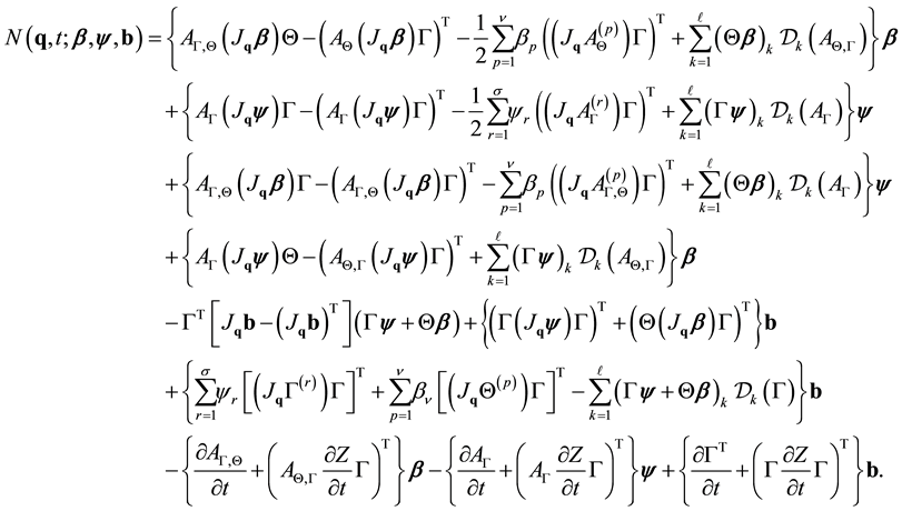
If on the one hand the use of quasi-velocities formally complicates calculations, on the other hand the final form of the system allows computing the equations merely by means of a list of particular matrices, once the Lagrangian function has been written and the quasi-velocities have been chosen.

We pay attention to keep separated the various contributions to the mobility of the system; the customary stationary case can be easily recovered from the general equations we will write.

An energy balance-type equation, which will be proposed in terms of the quasi-velocities, affirms the conservation of the energy in the full stationary case and shows the contributions of the different terms in the rheonomic context.

We will conclude by presenting some applications of the developed system of equations.

Most of the formal notation used onward is explained just below. For a given a list of variables,

the operator will compute the gradient of a scalar funcion, and calculates the Jacobian matrix of a vector:, ,.

Anywhere, vectors are in bold type and are meant as columns: row vectors will be written by means of the

transposition symbol. Moreover, is the null column vector, is the null matrix,

the null matrix and the unit matrix of size.

2. Modelling the System

The theoretical frame we point and expand is contained in [2] .

Let us consider a system of n point particles, , restricted both by geometrical constraints and by kinematic constraints, , ,:

(1)

(2)

where is the representative vector of the system and, for each fixed t, , is a matrix of size, a vector in. The constraint equations are assumed to be independent:

(3)

We first make use of the integer relations (1) in order to write the system configuration by means of the parametrisation, where, are the local Lagrangian coordi-

nates. The velocity of the system agrees with (1), but it must be consistent also with the

differential constraints (2) which are rewritten, in terms of the Lagrangian coordinates and of the generalized velocities, as

(4)

and in case of fixed constraints. The dynamics of the system is summarized in by, where represents the momentum of the system, , respectively all active forces and all constraint reactions (the i-th triplet concerning). The virtual displacements of the system at each time t and at each position are the vectors in such that [2]

(5)

giving in each, t the dimensional linear space

,

where are the rows of. At the same time, the assumption of smooth constraints make us write

(6)

where, are unknown multipliers.

The projection of the dynamics equation on the subspace generated by the vectors, (the

columns of), although such as space strictly includes, if, is anyhow noteworthy:

(7)

where we assumed and we defined the Lagrangian function

(8)

with symmetric and positive definite matrix of size and. The Equation (7) written for the unknown quantities, have to be considered together with the Equations (4).

In order to improve (7), we see from (4) and (5) that (virtual displacements) is the set of vectors

such that,.

Owing to (3) and recalling (4), it is, hence the solution of the come last linear system, which ex-

plicitly writes, is

(9)

with appropriate coefficients and arbitrary factors in,. We conclude that

, or, equivalently, the vectors, form a basis for.

At this stage, calling the matrix of size and elements and noticing that the columns of give the basis for, the projection of the dynamics equation on gives, by virtue also of (6):

(10)

where the effect of the nonholonomic constraints (through) on the ordinary Lagrangian equations for hol-

onomic systems is evident (in the absence of (2), say, both (10) and (7) are).

The differential Equation (10) are for the unknown quantities and they have to be combined together with the Equation (4). With respect to (7), they have the advantage of not exhibiting the multipliers.

Remark 2.1 Either Equation (7) or (10) can be employed not necessarily for discrete systems of point particles: once the Lagrangian coordinates have been selected and the Lagrangian function has been written, they can be the same calculated.

The expedience of introducing quasi-velocities (or pseudovelocities) which have to be chosen in a suitable way in order to disentangle the mathematical problem, is by custom performed in nonholonomic systems.

Following the adopted standpoint, the definition of the quasi-velocities steps in establishing a specific (and convenient) connection between and

(11)

where are required to guarantee that the square matrix of size is invertible. In

this way, each set of kinetic variables is linked to a singular set of quasi-velocities, and vice versa. More precisely, (11) and (4) give

(12)

where is the same as (9) and is a matrix. The first system in (12) shows both the selection on the coordinates of the tangent space necessary to fulfill the restrictions on the system’s velocity (leading to the subspace) and the kinematic conditions themselves.

In order to express (10) as a function of the variables, and to eliminate, it suffices to extract from (12)

(13)

and to define

(14)

where

(15)

By using the formulae (see (11))

(16)

where is the matrix whose elements are, for each,

we can write (10) in terms of the demanded variables (we use, see (12)):

(17)

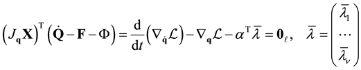
Remark 2.2 Multiplying both sides of (17) by and performing the customary steps leading to the energy balance one finds

(18)

In the stationary circumstance, , and the Legendre transform of is conserved.

Our next step is writing (17) explicitly, sorting the terms in a suitable way: we start from the calculation

(19)

so that (17) takes the structure

(20)

Provided that means the -th column of any matrix and defining for any the operation

(21)

for a matrix of size, the terms in (20) are defined by the following expressions, where means the -th component of any vector and:

Equation (20) is sorted on the strength of the quasi-velocities: is quadratic with respect to, is linear with respect to the same variables and does not contain.

Since A is a positive-definite square matrix and, even is a positive-definite

symmetric matrix. Hence, system (20) + (13) can be written in the normal form, where is

a list of functions, whose regularity allows us to apply the standard theorems on existence and uniqueness of solutions to first-order equations with given initial conditions.

Before commenting Equation (20), we remark that the entries of the matrix defined in (21) are, for each:

(22)

We see now that a certain number of significant cases are encompassed by (20):

・ merely geometric constraints, corresponding to, , so that (4) are not present and all the terms containing, and the related quantities must be dropped in (20). Furthermore:

○ selecting (quasi-velocities are the generalized velocities) in (11) and (13) means

so that in (20) are written with as

thus the Lagrangian equations for geometric constraints (bearing in mind (22))

, are achieved.

○ establishing (11) as 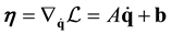(quasi-velocities are the generalized momenta) means

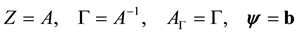
In this case (13) together with (20) are the Hamiltonian equations for

:

indeed the first one is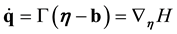, whereas (20) reduces to

(23)

with

(actually from one deduces and so that, also considering

, many terms are cancelled).

Since for any, it is

therefore (23) is, as stated.

・ Stationary case, where the different contributions producing the dependence on must be dropped. If one is dealing with a scleronomic system (covering many of common instances), the constraints (1), (2) reduce to

(24)

(25)

Conditions (24) entail and (if even the forces are independent of

time), on the other hand (25) implies.

Equation (11), if one reasonably chooses and independent of (otherwise, changes will be obvious), is. Since, system (20) + (13) drastically simplifies to

(26)

or, index by index, calling the entries of the matrix, and having in mind (22)

(27)

where is, for each index, the square matrix of order

Equations (27) are identified with the Boltzmann-Hamel Equations (17) for the Lagrangian function

(see [3] [4] ). In this case the Legendre transform is a first integral of

motion, see Remark 1.2.

・ Reduced Lagrangian function for geometric constraints: in case of ν cyclic variables, ,

(4) can play the role of the relations derived from the first integral of motion, ,

that is,. Assuming that, , it is possible

to acquire, according to (13), , , where, and b_j depend

only on. At this point, setting, , we have, with respect to (11) and (12), and (Kronecker’s delta),. Equation (20), which writes simply

, are the equations of motion for the reduced Lagrangian

,

with,; on the other hand, 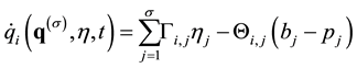for

, are the so called reconstruction equations.

3. Some Applications

We adopt now Equation (20) in order to formulate a couple of remarkable mechanical systems, each of them in a double form, as scleronomous and rheonomous model.

3.1. Pendulum on a Skate

Consider a system of four points, and equidistant and lying on a horizontal plane, equidistant from and, oscillating around, equidistant from and and coplanar to the latter points and (see Figure 1).

The system represents a simple model for the motion of a bicycle, as exhibited in [5] : the mass in is added on order to sketch the rigid structure of the bicycle (just as and represent the front and the back wheels), as well as the pendulum simulates the movement of a driver.

Let be a fixed point on the horizontal plane containing and, the ascending vertical versor, the midpoint of the segment and perpendicular to the same segment: the geometrical constraints (1) are written by means of the constant assigned values, , as

(28)

Since the constraints are independent and, we have,. Setting a fixed reference system and the angle between and, the angle between and, the angle between and, one defines the orthonormal versors

, ,

so that, , , and choose the five parameters as Lagrangian coordinates, where.

Opting for considering the segment as a rigid bar of mass M (instead of a discrete point system, although not significant), the Lagrangian function (8) is written with, , and

where is the total mass and

(29)

The only one kinetic constraint concerns with the velocity of the back “wheel”, to be aligned with the segment:

(30)

or, that is (4) for, ,.

Hence and the four quasi-velocities (11) are selected by setting

and.

Furthermore, (12) gives

so that

By computing the first line in (26) one finds the four equations of motion

joined with the conservation of the quantity.

3.2. Assignment of the Front Motion

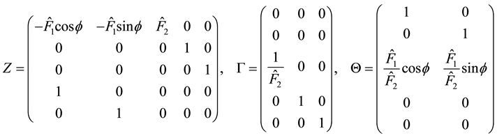
We modify the previous model by forcing the velocity of the front “wheel” to be a known function of time (a simpler version was considered in [6] for the motion of a bike):. With respect to (28), time enters explicitly the geometrical constraints and the fourth one has to be removed. Hence, in this example we have, , and we choose. The midpoint is located by 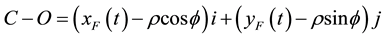and the Lagrangian function (8) is written with

, ,

whereas is the same function.

The constraint (30) is now, that is (4) for,. Choosing, we have simply

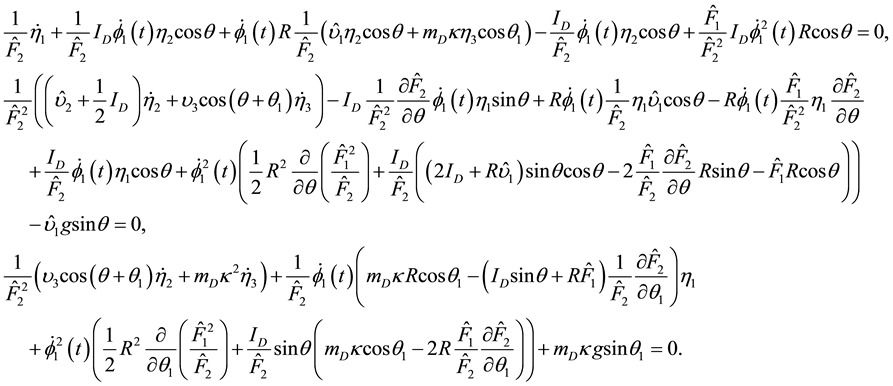
Equation (20) are written with

and correspond to

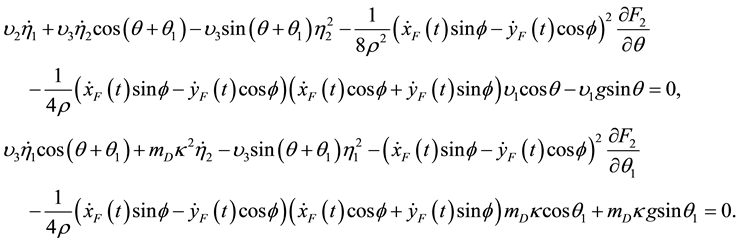
The energy balance (18) writes and the function in the right side of the latter equality is

with.

3.3. Rolling Disk with Pendulum

A different version of the model 3.1 lies in replacing the bar with a disk and obtaining the unicycle with rider model presented in [7] (see Figure 1 again, replacing the bar with the disk). The system we consider here is a disk of diameter and mass, in addition to the same points (with mass) and (with mass). We directly choose the coordinates (see Remark 2.1) where the new parameter is the angle of rotation of the disk around the axis perpendicular to the disk and passing through the centre. The Lagrangian function is written with and

where and (see (29))

The kinematic constraint of rolling without sliding entails the zero velocity of the contact point:

(31)

which is (4) with, and.

This time and the choice

leads to

where. Moreover

with

and the corresponding equations of motion (20) are

where

3.4. Assigned Rotational Velocity of the Disk

We finally consider the same system with the differential constraint (31), but assigned (we may think about an engine-driven motor bike or electric bike): in that case 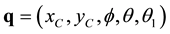and (4) is setted

with and,.

The Lagrangian fucntion (8) is written with A the same as in the previous Example 3.1, except for removing

the fourth row and the fourth column, and,. In the matter of (11), which has to be written for, if one defines the quasi-velocities,

, one gets and

Calculating the products in (15) gives

,

,

and the computation of (20) gives the three equations of motion

4. Conclusions

The paper aims at formulating a general scheme of equations for rheonomic mechanical systems exposed to either geometrical (1) and differential (2) constraints. We pay special attention to tell apart the different contributions due to the explicit dependence on time, deriving from the holonomous constrictions (via and of (8)), the nonholonomous constrictions (via of (4)) and the definition of quasi-velocities (via) of (11)).

Since the equations of motion are projected in the subspace of the velocities allowed by the constraints (both holonomous and nonholonomous), the Lagrange multipliers are absent from the equations.

The procedure proposed by (20) requires only calculation of the Jacobian matrix of vectors and the algebraic multiplication of matrices and vectors.

Making use of quasi-velocities renders the equations versatile to more than one formalism and, as it is known, the appropriate choice of them meets the target of facilitating the mathematical resolution of the problem.

The last point is part of the matters listed below and which will be dealt with in the future:

-Find an appropriate choice of the quasi-velocities in order to disentangle (20) from (13) as much as possible,

-Make use of the structure of the equations and of the properties of the various matrices involved in order to study the stability of the system,

-Take advantage of some peculiarity of the system in order to refine the set of equations and achieve information.

The latter subject is faced in [8] [9] for the stationary case by means of a robust and complex theory in connection with symmetries in nonholonomic systems.

References

- Poincaré, H. (1901) Sur une forme nouvelle des èquations de la méchanique. Comptes Rendus de l’Académie des Sci- ences, 132, 369-371.
- Gantmacher, F.R. (1975) Lectures in Analytical Mechanics. MIR.
- Maruskin, J.M. and Bloch, A.M. (2011) The Boltzman-Hamel Equations for the Optimal Control of Mechanical Systems with Nonholonomic Constraints. International Journal of Robust and Nonlinear Control, 21, 373-386. http://dx.doi.org/10.1002/rnc.1598
- Cameron, J.M. and Book, W.J. (1997) Modeling Mechanisms with Nonholonomic Joints Using the Boltzmann-Hamel Equations. Journal International Journal of Robotics Research, 16, 47-59. http://dx.doi.org/10.1177/027836499701600104
- Talamucci, F. (2014) The Lagrangian Method for a Basic Bicycle. Journal of Applied Mathematics and Physics, 2, 46- 60.
- Levi, M. (2014) Bike Tracks, Quasi-Magnetic Forces, and the Schrödinger Equation. SIAM News, 47.
- Zenkov, V., Bloch, A.M. and Mardsen, J.E. (2002) Stabilization of the Unicycle with Rider. Systems and Control Letters, 46, 293-302. http://dx.doi.org/10.1016/S0167-6911(01)00187-6
- Bloch, A.M., Krishnaprasad, P.S., Mardsen, J.E. and Murray, R. (1996) Nonholonomic Mechanical Systems with Sym- metry. Archive for Rational Mechanics and Analysis, 136, 21-99. http://dx.doi.org/10.1007/BF02199365
- Bloch, A.M., Mardsen, J.E. and Zenkov, D.V. (2009) Quasivelocities and Symmetries in Non-Holonomic Systems. Dy- namical Systems, 24, 187-222. http://dx.doi.org/10.1080/14689360802609344