Journal of Applied Mathematics and Physics
Vol.2 No.7(2014), Article
ID:46804,8
pages
DOI:10.4236/jamp.2014.27057
The Case of Nonzero Initial Conditions in the Evolution of the Charge Density Distribution Function for a Spherically Symmetric System
Boris I. Sadovnikov1, Alex A. Zhavoronkov2*
1Faculty of Physics, Moscow State University, Moscow, Russian
2Moscow Institute of Physics and Technology, Dolgoprudny, Russian
Email: *alex@biogerontology.org
Copyright © 2014 by authors and Scientific Research Publishing Inc.
This work is licensed under the Creative Commons Attribution International License (CC BY).
http://creativecommons.org/licenses/by/4.0/


Received 19 February 2014; revised 19 March 2014; accepted 25 March 2014
ABSTRACT
We explored the Cauchy problem for the evolution of the charge density distribution function for a spherically symmetric system with nonzero initial conditions. In our model, the evolution of the charge density distribution function is simulated for the case of a non-uniform charged sphere. The initial speed of the system is nonzero. The solution breaks down into two components: the first one describes the system’s motion as a whole and the second describes the process of the evolution of the charge density function under the influence of its own electric field in the center-of-mass system. In this paper we considered the characteristic features of the implementation of a difference scheme for numerical simulation. We also illustrate the process of “scattering” of a moving charged system under the influence of its own electric field on the basis of the solution of the Cauchy problem for vector functions of the electric field and vector velocity field of a charged medium.
Keywords
Cauchy Problem, Nonzero Initial Conditions, Charge Density Distribution

1. Introduction
The main principles for studying the behavior of systems of many charged particles are stated in works [1] -[3] . The method based on hydrodynamic approach [4] [5] was successful. In our prior work, we explored the Cauchy problem for the evolution of the charge density distribution function for a spherically symmetric system with zero initial conditions. We simulated the evolution of the charge density distribution function for both the case of a uniformly charged sphere with zero initial conditions and for the case of a non-uniform charged sphere [6] . Here we expand on our prior work and explore the case of nonzero initial conditions.
In this paper we consider the Cauchy problem for the evolution of the charge density distribution function for a spherically symmetric system with nonzero initial conditions for the velocity field  and nonzero initial conditions for the electric field vector
 .
.
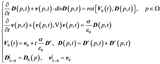 (1)
(1)
where  denotes the vector product of vectors
  and
and![]() ,
,  denotes the scalar product of vectors
  and
and![]() ;
; ![]() denotes the nabla differential operator;
denotes the nabla differential operator; ![]() denotes the dielectric constant of the vacuum and
denotes the dielectric constant of the vacuum and ![]() denotes constant initial velocity vector. The variable
denotes constant initial velocity vector. The variable ![]() corresponds to spatial coordinates
corresponds to spatial coordinates , and the variable
 ![]() represents time. Vector-function
represents time. Vector-function  denotes the electric field vector;
  is a vector field of medium speeds;
  is the external electric field;
  is the beam’s own electric field. The constant
 sets the ratio between the charge and the mass of the particles.
 ![]() represents the area, in which the solution of the system is being considered. This system, together with the initial conditions, leads to the formulation of the Cauchy Problem (1), the solution of which describes the evolution of the charge density distribution function under the influence of its own electric field.
represents the area, in which the solution of the system is being considered. This system, together with the initial conditions, leads to the formulation of the Cauchy Problem (1), the solution of which describes the evolution of the charge density distribution function under the influence of its own electric field.
2. Approximation of the Solution
The solution of Problem (1) may be found in the form of expanding vector functions of the electric field
 and vector functions of the velocity field
  into series:
 (2)
(2)
where the expansion coefficients in (2) can be expressed in terms of the derivatives of the initial conditions of Problem (1). Therefore, for the numerical solution of Problem (1), the approximation of the first three terms of Series (2) is to be considered. That is, for each time step, the approximation of the solution is obtained in the form of:
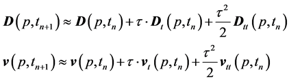 (3)
(3)
where ;
; ![]() is the total number of time steps;
is the total number of time steps;  is the step in the time
![]() . The coefficients of the time
. The coefficients of the time  in the first power are expressed in terms of the derivatives of
 ![]() and
and  of the previous step in time
  by formulas:
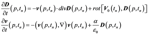 (4)
(4)
We have the same situation for the coefficients of the time ![]() in the second power:
in the second power:
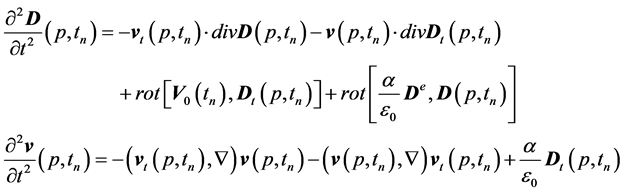 (5)
(5)
The values  and
and  are found using formulas (4). As a result, the formulas (3-5) can be used for the numerical solution to Problem (1). The difference scheme for spatial derivatives will be considered below.
3. An Example of the Numerical Solution
Let’s consider the case where the center of mass moves with a constant velocity . Due to the fact that the problem loses its symmetry and the value
  is nonzero, it is necessary to solve the complete formulation of Problem (1).
Let’s consider a charged sphere with a charge density function in the form of:
 , (6)
, (6)
where  is a normal logarithmic distribution;
 ![]() are constants;
are constants;  is a particle number.
Let’s solve the three-dimensional problem in the rectangular mesh. Suppose there is a three-dimensional area in which the problem is to be solved. To define the area, we take a parallelepiped with side lengths  as the geometric shape of the area. In this area we set a rectangular mesh
 (7)
(7)
in increments of , where
 ![]() is the number of partitions of
is the number of partitions of . We set a time mesh
 in increments of
 , where
 ![]() is a period of time, in which the problem is to be solved.
is a period of time, in which the problem is to be solved.
For numerical solution we use the first-order approximation in time and that is what we obtain
 (8)
(8)
We will use a different partition number of time increments. In other words, we will change the time increment from long to short, and we will see how the accuracy of the solution changes depending on the time increment. We will take the following value of the initial velocity:
 (9)
(9)
i.e. the movement along the axis OX. The time interval is , and the number of time increments NT will be changed in the range: 50, 100, 200, 400, and 800. Figure 1 shows the result of the final distribution of the charge density with the number of time increments NT = 50.
We can see a strong asymmetry of the distribution in the direction of movement.
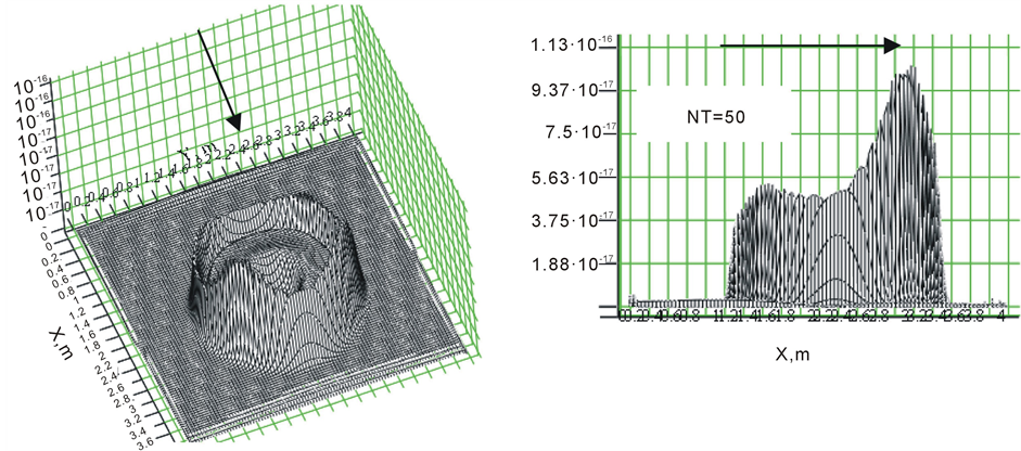
Figure 1. The final distribution of the charge density with the number of partitions in time NT = 50.
This result contains an artifact, since the symmetry of the distribution is breaking. Therefore, the time increment should be reduced. Figure 2 shows the sequence of such distributions which corresponds to a decreasing time increment. The arrow shows the direction of the velocity![]() .
.
Figure 2 shows that the first-order approximation in time requires a significant decrease in the time increment. To achieve the required accuracy we have to decrease the time increment in more than one order of time. In this regard, it will be interesting to do a similar calculation with the second-order approximation in time scheme.
Thus, we consider the second-order approximation in time using (3-5). Figure 3 shows the charge density distribution function calculated according to the difference scheme (3-5). So, when the number of partitions in time NT = 50 we get a result comparable to the number of NT = 800 for a first-order approximation in time scheme. This result significantly reduces the computation time.
However, there are other problems related to the accuracy of the difference scheme. One of them is that it doesn’t preserve the full charge. Let’s consider the charge density distribution along the direction of the system’s motion. The section of the graph in Figure 4 is shown with the white line. This fragment of the charge density distribution function is then enlarged in Figure 5, which shows the charge density distribution at various points of time along the section.
Figure 5 shows that there is an area where we can observe oscillations of the charge density function. The two areas enclosed by rectangles in which there is a violation of charge/mass conservation law. The first area is at the bottom. In the figure it is shown as a separate enlarged fragment. It is clearly seen that the charge density function changes its sign. The sign changes because the density value itself must be zero in this area. In the other area the density function is nonzero, that’s why there has been an increase of density value at the “wave border.”
Such behavior of the solution is incorrect in both cases. Although the difference scheme uses second-order approximation in the coordinate and the second-order approximation in time, the problem still cannot be solved by reducing increments.
This problem is not new among such kind of schemes, and can be solved by means of introduction of a scheme that takes into account the direction of the charge flow. In other words, we use another difference approximation of the derivative depending on the flow direction.
So, if the flow in the node is directed from left to right, then the derivative is approximated by the expression:
 (10)
(10)
if the flow in the node goes from right to left, the derivative can be written as:
 (11)
(11)
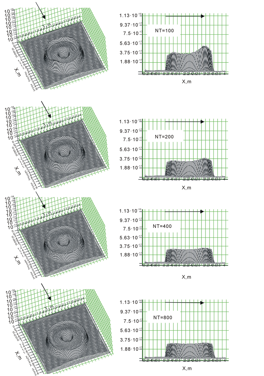
Figure 2. The reduction of density function error by reducing the time increment.
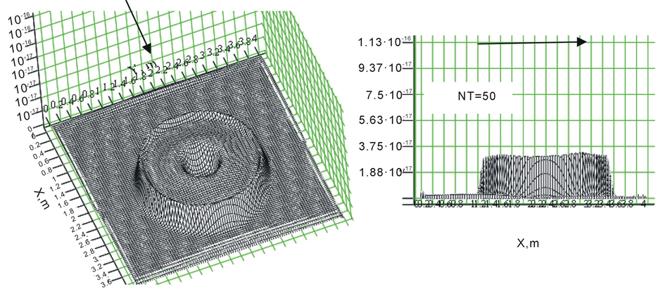
Figure 3. The charge density distribution for the second-order approximation in time scheme.
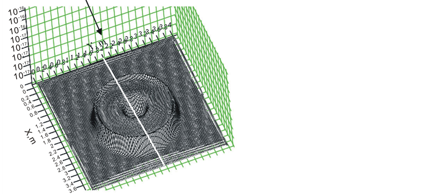
Figure 4. The charge density distribution for the second-order approximation in time scheme showing the position of the section of the graph further illustrated in Figure 5.
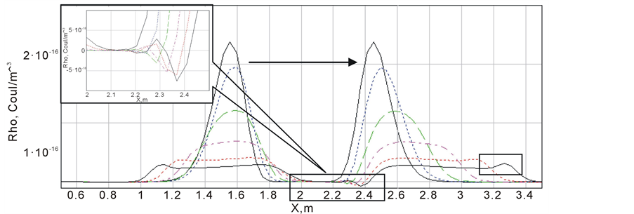
Figure 5. The enlarged fragment of the charge density distribution function.
Of course, the scheme has a coordinate order, so that the first order takes the place of the second one, but on the other hand, the problem of the oscillations of the charge density will be compensated. After using the approximations (10) and (11) the graph shown in Figure 5 takes the form of the graph shown in Figure 6. As seen from Figure 6 the problem of charge conservation has been solved both in the first and in the second area.
However, we had to sacrifice the difference scheme accuracy along the coordinate. This loss of accuracy was not wasted; because Figure 7(a) shows the dips in the charge density which appeared on the right and on the left of a moving clot, although there were none of them in the second-order coordinate. Therefore, to compensate for this effect, all we have to do is to increase the dimension of the mesh to 150 × 150 × 150 instead of 100 × 100 × 100. As a result, we can see that the dips in the charge density disappeared as shown in Figure 7(b).
4. Conclusions
The mathematical methods developed in this work may be applied in many areas ranging from theoretical physics to 3D graphics to machine learning in aging research [7] [8] .
In this paper we considered the collective effects, which influence the evolution of the beam charge density distribution function. The motion of a charged system influenced by its own electric field has been simulated. In this work we constructed the difference scheme for the Cauchy problem with different orders of approximation and provided the numerical calculations for the model charge density distribution, which illustrate the application of the obtained difference scheme.
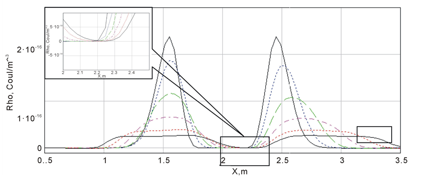
Figure 6. The evolution of the charge density function with time.
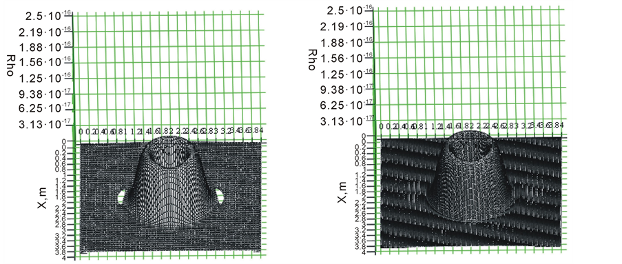
Figure 7. a), b) on different meshes: a) 100 × 100 × 100, b) 150 × 150 × 150.
Acknowledgements
We would like to thank Dr. Evgeny E. Perepelkin and Dr. Natalia G. Inozemtseva for developing the foundation of this research and for their help in preparing the paper. We also thank the reviewers for valuable comments and advice and the UMA Foundation for the help in preparation of this manuscript.
References
- Maslov, V.P. (1978) Equations of the Self-Consistent Field. Itogi Nauki i Tekhniki, Sovremennye Problemy Matematiki, 11, 153-234. http://dx.doi.org/10.1007/BF01084247
- Vlasov, A.A. (1968) Statistical Distribution Functions. Nauka, Moscow.
- Inozemtseva, N.G. and Sadovnikov, B.I. (1987) Evolution of Bogolyubov’s Functional Hypothesis. Physics of Particles and Nuclei, 18, 53.
- Harlow, F.H. (1963) The Particle-in-Cell Method for Numerical Solution of Problems in Fluid Dynamics. Proceedings of Symposium in Applied Mathematics, 15, 269.
- Harlow, F.H., Gryigoryan, S.S. and Shmyglevskiy, Y.D. (1967) The Particle-in-Cell Method for Numerical Solution of Problems in Hydrodynamics. Moscow, 383-386.
- Perepelkin, E., Inozemtseva, N. and Zhavoronkov, A. (2014) The Evolution of the Charge Density Distribution Function for Spherically Symmetric System with Zero Initial Conditions. World Journal of Condensed Matter Physics, 4, 33-38. http://dx.doi.org/10.4236/wjcmp.2014.41005
- Zhavoronkov, A. and Cantor, C.R. (2011) Methods for Structuring Scientific Knowledge from Many Areas Related to Aging Research. PLoS ONE, 6, e22597. http://dx.doi.org/10.1371/journal.pone.0022597
- Kolesov, A., Kamyshenkov, D., Litovchenko, M., Smekalova, E., Golovizin, A. and Zhavoronkov, A. (2014) On Multilabel Classification Methods of Incompletely Labeled Biomedical Text Data. Computational and Mathematical Methods in Medicine, 2014, 781807. http://dx.doi.org/10.1155/2014/781807
NOTES

*Corresponding author.