International Journal of Intelligence Science
Vol.2 No.4(2012), Article ID:23686,7 pages DOI:10.4236/ijis.2012.24012
Probability Elicitation in Influence Diagram Modeling by Using Interval Probability
1School of Management, Hefei University of Technology, Hefei, China
2Key Laboratory of Process Optimization and Intelligent Decision-Making, Ministry of Education, Hefei, China
Email: xiaoxuanhu@hfut.edu.cn
Received May 29, 2012; revised July 31, 2012; accepted August 10, 2012
Keywords: Influence Diagram; Probability Elicitation; Interval Probability; Decision-Making
ABSTRACT
In decision modeling with influence diagrams, the most challenging task is probability elicitation from domain experts. It is usually very difficult for experts to directly assign precise probabilities to chance nodes. In this paper, we propose an approach to elicit probability effectively by using the concept of interval probability (IP). During the elicitation process, a group of experts assign intervals to probabilities instead of assigning exact values. Then the intervals are combined and converted into the point valued probabilities. The detailed steps of the elicitation process are given and illustrated by constructing the influence diagram for employee recruitment decision for a China’s IT Company. The proposed approach provides a convenient and comfortable way for experts to assess probabilities. It is useful in influence diagrams modeling as well as in other subjective probability elicitation situations.
1. Introduction
An influence diagram (ID) [1] is a directed acyclic graph for modeling and solving decision problems under uncertainty. It provides a more compact way to represent complex decision situations than a decision tree does. In recent years, influence diagrams have been used as effective modeling tools for Bayesian decision analysis.
The work of constructing an influence diagram can be divided into two sub-works: The first one is to build the influence diagram structure; the other one is to assign parameters to all kinds of nodes, including assigning conditional probabilities for chance nodes, acquiring the utilities for value nodes and generating decision alterna-tives for decision nodes. The whole work is challenging and time consuming, and a number of difficulties may be faced. Bielza et al. have discussed the important issues in modeling with influence diagrams [2-4].
During the entire construction process, the assignment of conditional probabilities for chance nodes is considered the most difficult problem. There are two common used solutions to get probability values: learning from data or acquiring from experts. In the machine learning community, many algorithms have been presented to learn probabilities from data [5-7]. However, in many real-world applications, we do not have available data set and have to elicit probabilities from experts. The probabilities are thus called subjective probabilities.
To deal with the imprecision and inconsistence of subjective probabilities, quite a few methods are developed to guide experts correctly giving probabilities, such as using visual tools like probability scale [8], probability wheel [9] and scaled probability bar [10], adapting Analytic Hierarchy Process (AHP) [11]. Wiegmann gives an overview of the popular elicitation methods [12].
In this paper, we focus on probability elicitation for influence diagrams. We present a new approach to elicit probabilities from experts. Our approach does not require experts to give point-valued probabilities but to give interval-valued probabilities instead. Because in daily life, it is unrealistic to expect experts to provide exact values of many probabilities. They are used to describing probabilities by verbal or other inexact expressions, such as “possible”, “rare” or “likely”. Each expression is an imprecise or fuzzy description of probability that actually means an interval of probability. Cano and Moral pointed out that imprecise probability model such as interval probability is more useful than exact probability model in many situations [13]. The experts would be more confident and feel more comfortable to deal with intervals probabilities. So, we apply the concept of interval probability [14-18] to elicit probabilities, and we combine multiple experts’ judgments to increase the accuracy of the final results.
The paper is organized as follows: In Section 2, we briefly introduce influence diagrams. Section 3 shows the basic concept of interval probabilities. In Section 4, we describe our approach of probabilities elicitation from experts. First we introduce the entire process of the approach, and then give the details of each step. In Section 5, we illustrate our approach by a real application: establishing an influence diagram model for employee recruitment decision for a China’s IT company. Finally, we give a conclusion in Section 6.
2. Influence Diagram
An influence diagram can be defined as a four-tuple [19]
such that1) G = (V, E) is a directed acyclic graph (DAG), with nodes V and edges E. V are partitioned into three sets, V = . VC, VD and VU are the set of chance nodes, decision nodes and value nodes, respectively. The dependence relations and information precedence among all the nodes are encoded in E.
2) X is a set of variables. X = , XC is a set of random variables, and each variable in XC is represented by a chance node of G. XD is a set of decision variables, and each variable in XD is represented by a decision node of G .
3) Pr is a set of conditional probability distributions. Each random variable  associates with a distribution
 .
.
4) U is a set of utility functions. Each value node  contains one utility function u(Xpa(vi)).
In influence diagrams, the chance nodes are represented by circulars, and each chance node associates with a probability distribution. The decision nodes are rectangles. Each decision node has a set of alternatives. The value nodes are diamonds. The parameters of each value node show the utility of various outcomes according to the decision makers. Directed arcs in influence diagrams have different meanings. Arcs pointing to decision nodes are called information arcs, which indicate information precedence. An information arc from a chance node A to a decision node B denotes that variable A will be observable before the decision is made. Arcs pointing to chance nodes are called relevance arcs, which represent the dependency between the variables and their parents. The missing arc between two chance nodes means conditional independence.
An example of an influence diagram is shown in Figure 1. Bob is going to decide whether to go to watch a football game tomorrow. The only factor he considering is the weather. If there is no rain, he will go; otherwise he prefers to stay at home. He has a weather forecast sensor, from which he can know whether it will rain or not tomorrow. But the sensor has a small probability to make wrong forecast. As shown in Figure 1, there is an information arc from the node “weather forecast” to the decision node, and a relevance arc from the node “weather forecast” to the node “weather”. Bob’s utility varies with various instances of decisions and weather conditions.
The evaluation of an influence diagram is to find the best alternative by comparing the expected utility (EU) among every decision alternatives. Suppose Dj is a decision node with a set of decision alternatives . First we calculate the EU of each decision alternative di:
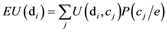 (1)
(1)
in which e represents the evidences.
Then we select the best alternative d* in , which satisfies
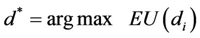 (2)
(2)
The original evaluation approach is to unfold an influence diagram into a decision tree. Obviously it is inefficient. Shachter presents a way to evaluate influence diagrams with two operations: node-removal and arcreversal [20]. By recursively using the two operations, an influence diagram is transformed into a diagram with only a utility node. The utilities for individual decision alternatives are computed during the process. F. Jensen et al. describe a way to convert an influence diagram into a junction tree [21], and then the message passing algorithm is operated on the junction tree for calculating the expected utility. Zhang describes a method to reduce influence diagrams evaluation into Bayesian network inference problems [22], so that many Bayesian network inference algorithms can be used to evaluate influence diagrams.
3. Interval Probability
The theory of imprecise probability has received much attention [13-17,23-26]. Interval probability is a major expression of imprecise probability that has been used in uncertain reasoning [14,18], decision making [15,16], and some other applications. It is an extension of classical probability so that can be adapted in more complex uncertain situations.
Definition 1. (Interval probability) [14,17,27]: Let Ω be
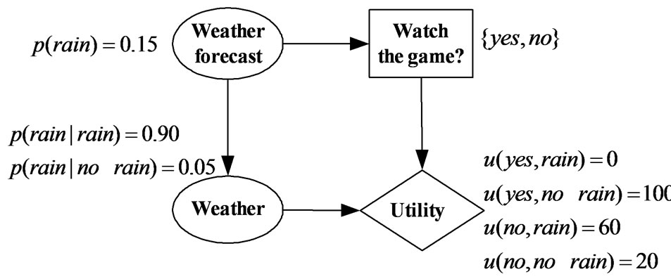
Figure 1. An influence diagram.
a sample space,  be a σ-field of random events in Ω,a set of intervals
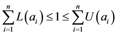
  is called interval probabilities if it satisfies the following conditions:
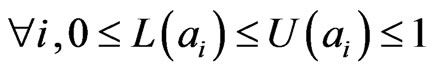 (3)
(3)
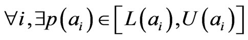 , such that
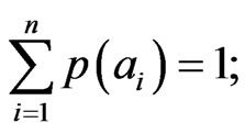 (4)
(4)
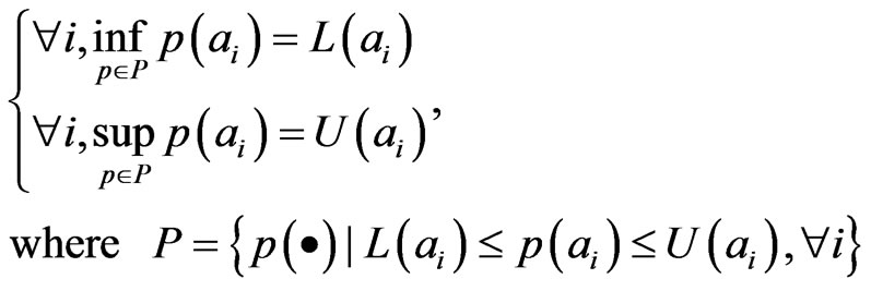 (5)
(5)
The intervals satisfy conditions (3)-(5) are also called reachable probability intervals [14] or F-probability [17].
Condition (4) can be modified as:
 (6)
(6)
Condition (6) and (4) are equivalence, while (6) is easier to understand. Condition (5) can be modified as [14,16]:
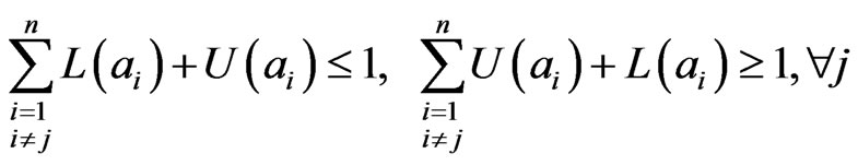 (7)
(7)
Condition (7) is a more strict constraint than (6).
4. Probability Elicitation
4.1. The Process of Probability Elicitation
Figure 2 shows the entire process of probability elicitation from multiple experts. It consists of four main steps. In the first step we select a group of appropriate experts in related domains. Then in the second step we elicit interval probabilities from the selected experts. In step 3, we combine different interval probabilities to form a single interval probability distribution. The linear opinion pool approach is adapted to complete the combination. In the last step, the interval probabilities are converted into point-valued probabilities, because only point-valued probabilities are recognized by influence diagrams. We deal with the conversion by a maximum entropy principle.
4.2. Selection of Experts
The elicitation work begins with selection of a group of appropriate experts. Each selected expert should meet the following four criteria: 1) Have to be specialists in the relevant fields; 2) Should be familiar with probability thinking and probability language; 3) Should have good communication skills so as to clearly express his opinion; 4) Should be quite patient to take time to engage in the
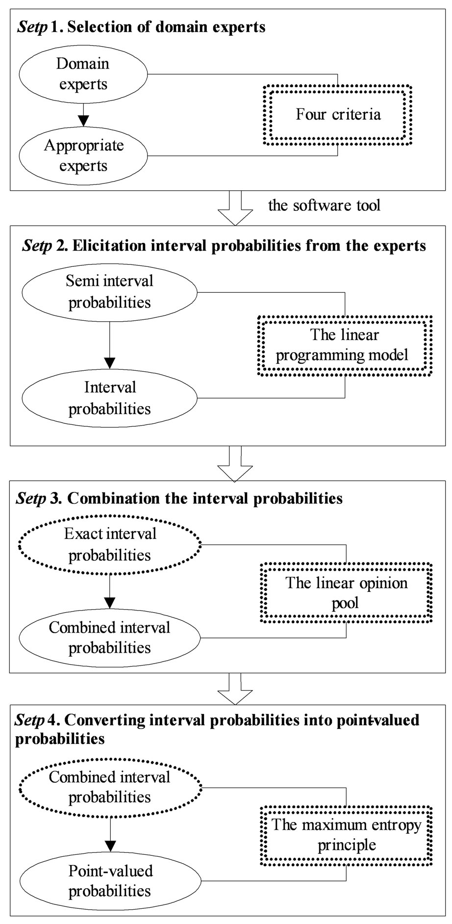
Figure 2. The process of probability elicitation.
modeling task.
The number of experts depends on the complexity of the influence diagram model, however, at least 3 experts should be guaranteed.
4.3. Interval Probability Elicitation
To help experts make judgments, we develop a software tool. The main window of the tool is shown in Figure 3. Two probability scales are arranged on the window. The above one is used to decide the lower bound of interval probability and the below one is used to decide the upper bound. The experts can drag the slider thumb on the scales to change the probability.
Using the tool, experts can rapidly assign intervals to
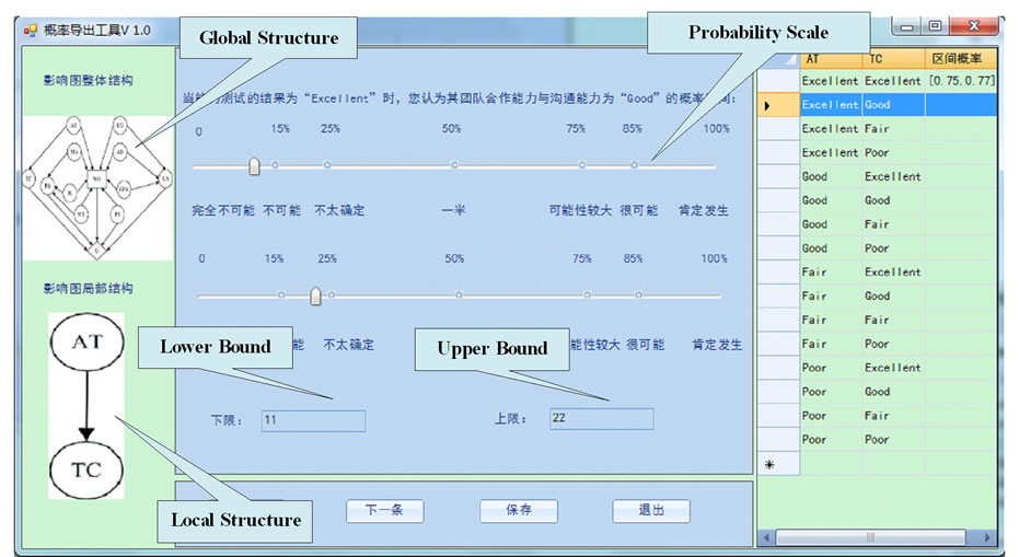
Figure 3. The software tool for eliciting interval probability.
probabilities. We denote them by and call them semi interval probabilities. Then we need to check if
  fully meet the definition of interval probabilities. If not, we use the following linear programming model [16] to elicit interval probabilities
  from
from  with least change.
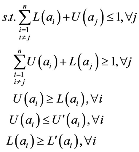 (8)
(8)
The model ensures
 and at the same time keeps the interval
 as big as possible. For example, the intervals on a random event are {[0.35, 0.40], [0.20, 0.30], [0.40, 0.45], [0.01, 0.05]}. The interval probabilities elicited from them are {[0.35, 0.39], [0.20, 0.24], [0.40, 0.44], [0.01, 0.05]}.
4.4. Interval Probability Combination
In order to improve the accuracy of the probabilities values, we elicit probabilities from multiple experts. Each expert assigns interval probabilities to chance nodes individually, and then their opinions are aggregated. By using multiple experts, we may get more precise results and eliminate the biasing effects.
A number of methods have been proposed for prob-ability combination. Here we take the linear opinion pool method [24,28]. The result is a linear combination of all the probability distributions given by different experts. The linear opinion pool is a simple but very useful method to combine probabilities. It allows us to assign weights to the experts. The weight is a scale for reflecting the difference of expertise. An expert with larger weight would have greater influence on the final results.
Let 
 are interval probability distributions of a discrete random variable A that assigned by expert j. Define
  as weighted sum of all the distributions:
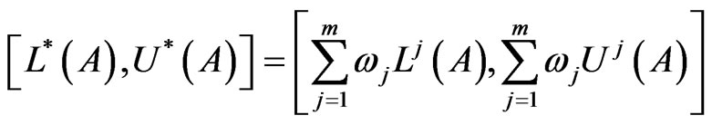 (9)
(9)
where  is the weight of expert j that satisfies
 .
.
Proposition 1.  is an interval probability distribution.
For combination, the important thing is to assign proper weight to each expert. Since the probabilities are subjective, some experts’ judgments may be more precise than the others. They should have greater influence on the final result. So the weight of individual expert should reflect the degree of expertise and would be different.
In most group decision-making situations, the weights are subjective. Here we propose a method to assign weights objectively. In detail, we give the weight to an expert by measuring the average distance (AL) between the probability distribution given by him and the distributions given by others. The value of AL shows the average similarity between a certain probability distribution and the other distributions. We consider if an expert’s judgment is closer to the most experts’ judgments, we assign him a higher weight; otherwise we assign him a lower weight.
Definition 2. The distance between two interval probability distributions
 and
and  is defined as
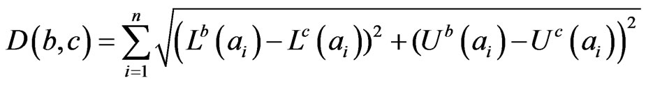 (10)
(10)
Definition 3. The average distance between an interval probability distribution and all the other distributions
 is defined as
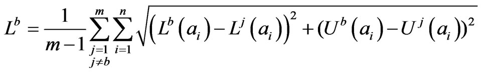 (11)
(11)
Definition 4. The weight  of expert b is defined as
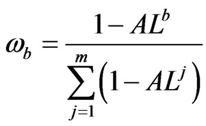 (12)
(12)
4.5. Convert Interval Probability into Point-Valued Probability
The evaluation algorithms of influence diagrams are all based on point-valued probabilities. After combination, we need to convert interval probability into point-valued probability. By definition 1, we know that there always exists point-valued probability distributions P(A) for each interval probability distribution [L(A), U(A)]. However, P(A) is not unique. In case we have no additional information, the most reasonable converting method is to use maximum entropy principle [15,29]. As shown below, the point-valued probability distribution is the solution of the linear programming model.
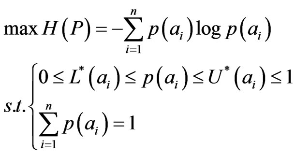 (13)
(13)
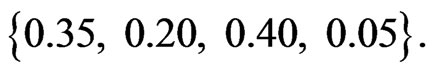
For example, the interval probability distribution is
 Then the point-valued probability elicited from it is
5. Case Study
A China’s IT Company is going to hire employees from several candidates who are all recent graduates. The company will make the decision after assessing individual ability of the candidates. On the basis of analysis on the relevant factors, we construct an influence diagram model, as shown in Figure 4. The nodes of the model are explained in Table 1.
After building the structure of the influence diagram, we consider the parameters of the nodes. We start with the conditional probability distribution of node “TC”. “TC” represents the teamwork spirit and communication skill of candidates. The company tests “TC” of candidates through a test and ranks it with four grades: “Excellent”, “Good”, “Fair” and “Poor”. However, the result of the test does not always according with the real performance. The conditional probability  represents the degree of the deviation.
For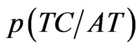 , we need to obtain sixteen probabilities, as shown in Table 2.
Here we illustrate the elicitation process of p(a1) to p(a4). We select five experts. By using the software tool, the semi interval probabilities given by each expert are shown in Table 3.
Using model (8), we transform them into real interval probabilities, which are shown in Table 4.
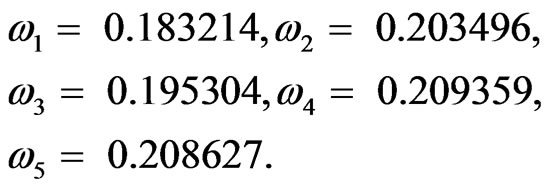
The weights of the experts obtained by formula (12)
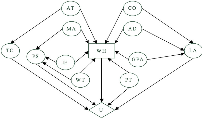
Figure 4. Influence diagram for employee recruitment.
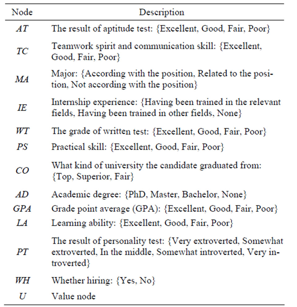
Table 1. The description of the nodes.
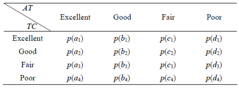
Table 2. Conditional probability table of node “TC”.
are listed as follows:
The combined interval probabilities obtained by formula (9) are shown in Table 5.
At last, we convert interval probabilities into pointvalued probabilities by using model (13). The results are shown in Table 6.
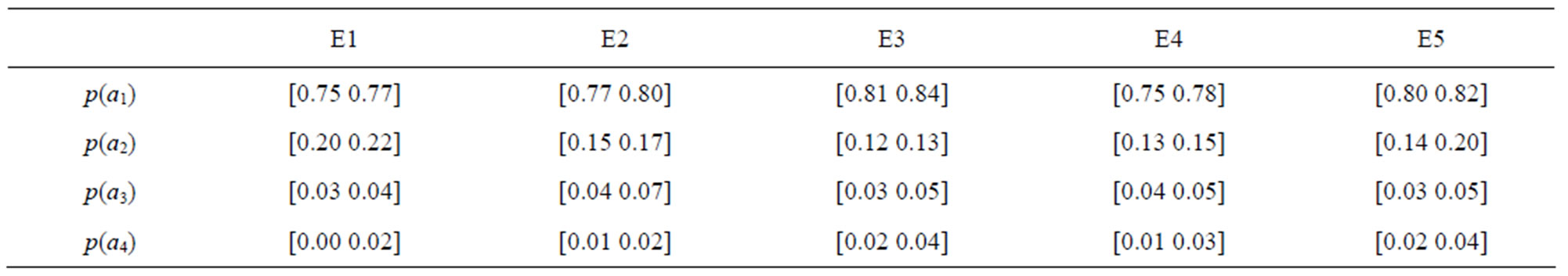
Table 3. Semi interval probabilities.
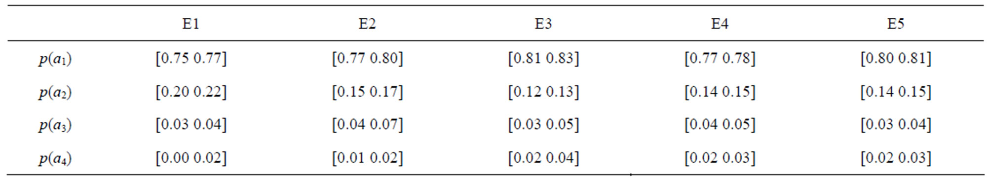
Table 4. Interval probabilities.
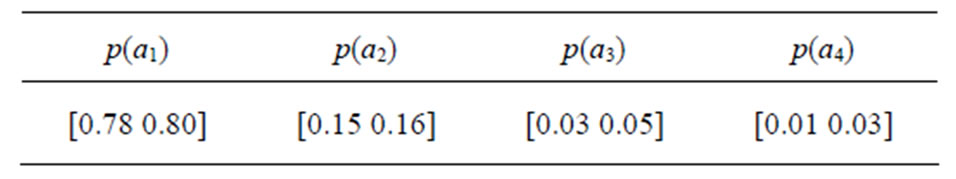
Table 5. The combined interval probabilities.
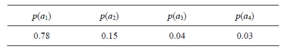
Table 6. The point-valued probabilities.
6. Conclusion
Influence diagrams have been widely used for decision analysis under uncertainty. The major obstacle of building an influence diagram is that it is difficult to get probabilities for chance nodes. Learning probabilities from data is a good approach but is useless in case of no available data set. In this paper, we propose a method to elicit probabilities from a group of domain experts. The theory of interval probability is adapted to handle the fuzziness of experts’ knowledge. Using a software tool, the experts assign interval probabilities to chance nodes, and then their judgments are combined. Finally, by using maximum entropy principle, the interval probabilities are converted into point-value probabilities. With this method, experts feel more comfortable and confident to make judgments. We believe this method is useful in influence diagrams modeling as well as in other probability elicitation situations.
7. Acknowledgements
This research was mainly supported by the National Natural Science Foundation of China (No. 70801024, 71001032).
REFERENCES
- R. A. Howard and J. E. Matheson, “Influence diagrams” In: R. A. Howard and E. M. James, Ed., Readings on the Principles and Applications of Decision Analysis, Menlo Park, 1983, pp. 719-763.
- C. Bielza, M. Gómez, S. Ríos-INsua and J. A. F. D. Pozo, “Structural, Elicitation and Computational Issues Faced When Solving Complex Decision Making Problems with Influence Diagrams,” Computers & Operations Research, Vol. 27, No. 7-8, 2000, pp. 725-740. doi:10.1016/S0305-0548(99)00113-6
- C. Bielza, M. Gómez and P. P. Shenoy, “Modeling Challenges with Influence Diagrams: Constructing Probability and Utility Models,” Decision Support Systems, Vol. 49, No. 4, 2010, pp. 354-364. doi:10.1016/j.dss.2010.04.003
- C. Bielza, M. Gómez and P. P. Shenoy, “A Review of Representation Issues and Modeling Challenges with Influence Diagrams,” Omega, Vol. 39, No. 3, 2010, pp. 227-241. doi:10.1016/j.omega.2010.07.003
- G. F. Cooper and E. Herskovits, “A Bayesian Method for the Induction of Probabilistic Networks from Data,” Machine Learning, Vol. 9, 1992, pp. 309-348. doi:10.1007/BF00994110
- S. L. Lauritzen, “The EM Algorithm for Graphical Association Models with Missing Data,” Computational Statistics & Data Analysis, Vol. 19, No. 2, 1995, pp. 191- 201. doi:10.1016/0167-9473(93)E0056-A
- D. Heckerman, “Bayesian Networks for Data Mining,” Data Mining and Knowledge Discovery, Vol. 1, No. 1, 1997, pp. 79-119. doi:10.1023/A:1009730122752
- S. Renooij and C. Witteman, “Talking Probabilities: Communicating Probabilistic Information with Words and Numbers,” International Journal of Approximate Reasoning, Vol. 22, 1999, pp. 169-194. doi:10.1016/S0888-613X(99)00027-4
- C. S. Spetzler and C. S. S. von Hostein, “Probability Encoding in Decision Analysis,” Manage Science, Vol. 22, No. 3, 1975, pp. 340-358. doi:10.1287/mnsc.22.3.340
- H. Wang, D. Dash and M. J. Druzdzel, “A Method for Evaluating Elicitation Schemes for Probabilistic Models,” IEEE Transactions on Systems Man and Cybernetics, Part B—Cybernetics, Vol. 32, No. 1, 2002, pp. 38-43. doi:10.1109/3477.979958
- S. Monti and G. Carenini, “Dealing with the Expert Inconsistency in Probability Elicitation,” IEEE Transactions on Knowledge and Data Engineering, Vol. 12, No. 3, 2000, pp. 499-508. doi:10.1109/69.868903
- D. A. Wiegmann, “Developing a Methodology for Eliciting subjective Probability Estimates during Expert Evaluations of Safety Interventions: Application for Bayesian Belief Networks,” Aviation Human Factors Division, University of Illinois at Urbana-Champaign, 2005. http://www.humanfactors.uiuc.edu/Reports&PapersPDFs/TechReport/05-13.pdf
- A. Cano and S. Moral, “Using Probability Trees to Compute Marginals with Imprecise Probabilities,” International Journal of Approximate Reasoning, Vol. 29, No. 1, 2002, pp. 1-46. doi:10.1016/S0888-613X(01)00046-9
- L. M. de Campos, J. F. Huete and S. Mora, “Probability Intervals: A Tool for Uncertain Reasoning,” International Journal of Uncertainty Fuzziness and Knowledge-Based Systems, Vol. 2, No. 2, 1994, pp. 167-196. doi:10.1142/S0218488594000146
- R. R. Yager and V. Kreinovich, “Decision Making under Interval Probabilities,” International Journal of Approximate Reasoning, Vol. 22, 1999, pp. 195-215. doi:10.1016/S0888-613X(99)00028-6
- P. Guo and H. Tanaka, “Decision Making with Interval Probabilities,” European Journal of Operational Research, Vol. 203, 2010, pp. 444-454. doi:10.1016/j.ejor.2009.07.020
- K. Weichselberger, “The Theory of Interval-Probability as a Unifying Concept for Uncertainty,” International Journal of Approximate Reasoning, Vol. 24, 2000, pp. 149- 170. doi:10.1016/S0888-613X(00)00032-3
- J. W. Hall, D. I. Blockley and J. P. Davis, “Uncertain Inference Using Interval Probability Theory,” International Journal of Approximate Reasoning, Vol. 19, 1998, pp. 247-264. doi:10.1016/S0888-613X(98)10010-5
- U. B. Kjaerulff and A. L. Madsen, “Bayesian Networks and Influence Diagrams: A Guide to Construction and Analysis,” Springer, Berlin, 2007.
- R. D. Shachter, “Evaluating Influence Diagrams,” Operations Research, Vol. 34, No. 6, 1986, pp. 871-882. doi:10.1287/opre.34.6.871
- F. Jensen, F. V. Jensen and S. L. Dittmer, “From Influence Diagrams to Junction Trees,” Proceeding of the Tenth Conference on Uncertainty in Artificial Intelligence, Seattle, 1994, pp. 367-373.
- N. L. Zhang, “Probabilistic Inference in Influence Diagrams,” Proceedings of the 4th Conference on Uncertainty in Artificial Intelligence, Madison, Wisconsin, 1998, pp. 514-522.
- R. F. Nau, “The Aggregation of Imprecise Probabilities,” Journal Of Statistical Planning and Inference, Vol. 105, 2002, pp. 265-282. doi:10.1016/S0378-3758(01)00213-0
- S. Mora and J. D. Sagrado, “Aggregation of Imprecise Probabilities,” In: B. Bouchon-Meunier, Ed., Aggregation and Fusion of Imperfect Information, Physica-Verlag, Heidelberg, 1997, pp. 162-168.
- F. G. Cozman, “Graphical Models for Imprecise Probabilities,” International Journal of Approximate Reasoning, Vol. 39, No. 2-3, 2005, pp. 167-184. doi:10.1016/j.ijar.2004.10.003
- P. Walley, “Towards a Unified Theory of Imprecise Probability,” The 1st International Symposium on Imprecise Probabilities and Their Applications, Ghent, 1999.
- T. Augustin, “Generalized Basic Probability Assignments,” International Journal of General Systems, Vol. 34, No. 4, 2005, pp.451-463. doi:10.1080/03081070500190839
- R. T. Clemen and R. L. Winkler, “Combining Probability Distributions from Experts in Risk Analysis,” Risk Analysis, Vol. 19, No. 2, 1999, pp. 187-203. doi:10.1111/j.1539-6924.1999.tb00399.x
- V. Kreinovich, “Maximum Entropy and Interval Computations,” Reliable Computing, Vol. 2, No. 1, 1996, pp. 63-79. doi:10.1007/BF02388188