Open Journal of Acoustics
Vol. 3 No. 2A (2013) , Article ID: 33434 , 9 pages DOI:10.4236/oja.2013.32A003
Trade-Off between Bandwidth and Number of Array Elements in the Performance Enhancement of Passive Fathometer
School of Engineering and Information Technology, University College, University of New South Wales, Canberra, Australia
Email: m.alam@adfa.edu.au
Copyright © 2013 Jahangir Alam et al. This is an open access article distributed under the Creative Commons Attribution License, which permits unrestricted use, distribution, and reproduction in any medium, provided the original work is properly cited.
Received April 19, 2013; revised May 19, 2013; accepted May 26, 2013
Keywords: Passive Fathometer; Cross-Correlation; SNR; Resolution; Bandwidth; Array Processing
ABSTRACT
Improved signal to noise ratio (SNR) and resolution of the ambient noise cross-correlation function (NCF) between two points help in the estimation of bottom profile of the ocean. One of the main requirements of the improvement of the SNR and resolution is collection of a large amount of data. These large amounts of data can be achieved by recording a large bandwidth ambient noise or using an array of hydrophones. This paper evaluates the performance of the array processing and compares it to the large bandwidth technique in terms of SNR and resolution of NCF. It is shown that the large bandwidth technique gives better SNR and resolution compared to the array processing technique under certain conditions. The outcome of this article finds application in the enhanced estimation of the passive fathometer.
1. Introduction
Time domain cross-correlation between two ambient noise fields plays an important role in the various estimation applications such as bottom profiling of the ocean [1,2], geoacoustic inversion [3] and finding critical angle at the water sediment interface [4]. Improved signal to noise ratio (SNR) and resolution of the ambient noise cross-correlation function (NCF) enhances all these estimations because it helps in the estimation of the Green’s function (GF) [2]. A large collection of data is an important requirement for the better estimation of the GF and thus improvement of the SNR and resolution of the NCF [2,5].
There have been significant numbers of work [4-7] related to the collection of coherent signals during the estimation of GF. Previous literature [4] shows that achieving the requirement of a sufficient amount of data using only two sensors requires a long observation time. The use of an array of hydrophones solves the problem of time constraints by averaging the results of each pair of hydrophones in the array [1,4,8,9]. The SNR and resolution are improved in the array processing but at the cost of complex signal processing and increased expenses [1]. Recent work [2] shows that increase of the bandwidth of the ambient noise field coming from the end-fire region improves SNR and resolution of the NCF even if noise fields are recorded at only two sensors.
In this paper, it is shown theoretically that the large bandwidth technique gives better SNR and resolution compared to the array processing technique under a wide range of circumstances. A mathematical derivation of the cross-correlation function in the array processing is presented here. Delay and sum (DS) beam-forming technique described in [1] is applied in the array processing of this paper, which leads to the derivation of the SNR and resolution of the NCF in array processing. A relationship between the two techniques is shown in this paper in which the resources required to achieve a desired SNR and resolution are defined.
This article is divided into six sections. Section two presents the background of array processing technique and section three provides the mathematics of the SNR and resolution of the cross-correlation function in array processing. Section four shows the numerical simulation of array processing technique to justify the mathematics of section three. Section five presents the comparison between the large bandwidth and array processing technique and finally section six summarises the findings and conclusions drawn from this study.
2. Array Processing
An array in the underwater signal processing is a collection of vertically or horizontally spaced hydrophones, that is used to acquire data at all the hydrophones simultaneously. The array is used in data acquisition applica tions to make use of beam-forming. Beam-forming is a signal processing technique that superimposes a number of time delayed signals by proper delay adjustment so that the SNR of the resultant signal increases [1,9]. Figure 1 shows an equispaced 4-hydrophone vertical array where hydrophones are noted by  and
and .
.  is placed in the top (towards ocean surface) and
  is placed in the bottom (towards seabed) of the hydrophone chain.
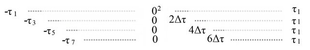
In this paper, it is assumed that the array is placed underwater and a noise signal coming from a surface noise source N which is placed in the end-fire region of the array. Each hydrophone of the array receives a direct path signal and a bottom reflected signal from A with corresponding time delays. Beam-forming the crosscorrelation of each pair of hydrophones, a strong correlation function can be achieved [1]. In the first stage of beam-forming, each hydrophone is taken as reference and cross-correlation is performed with all other hydrophones. All of these correlations are averaged together after proper delay adjustment so that desired peak of each correlation function coincides in the same position [1]. Figure 2 shows the conceptual diagram of the positions of correlation peaks in every correlation steps of the first stage of beam-forming.
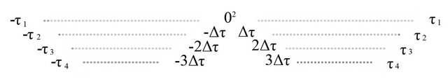
Figure 2(a) shows that the cross-correlations between the reference hydrophone  and all other hydrophones generate correlation peaks in different positions. First row of Figure 2(a) shows the autocorrelation of the noise field received by
  where the leftmost and rightmost peaks are generated at
 ![]() distance from the correlation centre (0 position) due to the cross-correlation between
distance from the correlation centre (0 position) due to the cross-correlation between
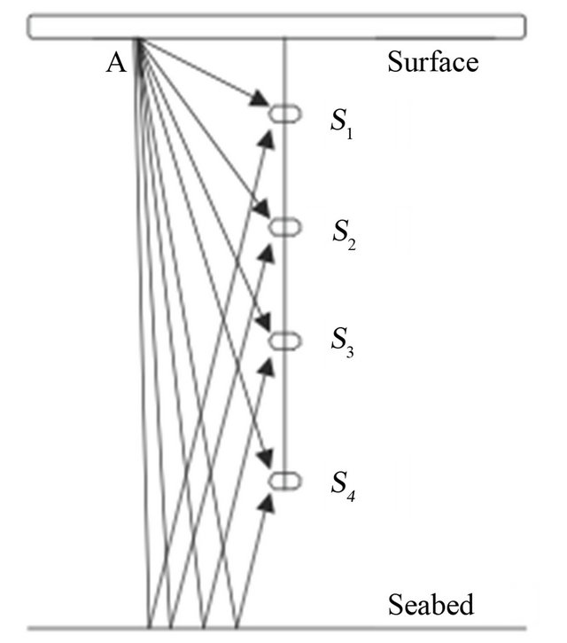
Figure 1. Hydrophone array.
 (a)
(a)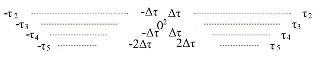 (b)
(b)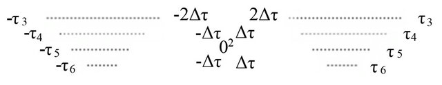 (c)
(c) (d)
(d)
Figure 2. Position of the peaks in the cross-correlation between reference and other hydrophones; (a) Reference hydrophone S1; (b) Reference hydrophone S2; (c) Reference hydrophone S3; (d) Reference hydrophone S4.
direct and reflected signals. ![]() is the delay difference between the direct and reflected signals of
is the delay difference between the direct and reflected signals of . Two other peaks coincide in the centre of the correlation where one is produced because of the correlation between direct signals and other for the reflected signals. In the cross-correlation between
  and
and  as shown in the second row of Figure 2(a), the leftmost and rightmost peaks are shifted towards centre by
  and two centre peaks are shifted away from the centre by the same amount where
  is the time delay between two consecutive hydrophones. In case of the cross-correlations shown in third and fourth rows of Figure 2(a), the peaks are further shifted by
  and
and![]() respectively. This is because direct signals come later and reflected signals comes earlier to the bottom hydrophones compared to the top hydrophones [1]. The position variables
respectively. This is because direct signals come later and reflected signals comes earlier to the bottom hydrophones compared to the top hydrophones [1]. The position variables ![]() can be expressed in terms of
can be expressed in terms of ![]() and
and  as follows
The superscript of a position describes the number of peaks that coincide in that position. For example  describes
 ![]() number of peaks superimpose in
number of peaks superimpose in  position of the correlation. The Figures 2(b)-(d) represent the position of the peaks of the correlations considering the reference hydrophones
  and
and  respectively.
In the first stage of beam-forming, the correlated signals need to be time-shifted and then averaged. The rightmost and leftmost peaks are very important in fathometer application [1,3]. Any of these two peaks can be chosen in the array processing for depth estimation as they produce same result. If the rightmost peak of the correlation is the point of interest, the correlation peaks shown in the second to fourth rows of Figures 2(a)-(d) need to be right-shifted by  and
and ![]() respectively so that the rightmost peaks of the correlations of each figure coincide in the same position. The first to fourth row of Figure 3 show the time-shifted correlation signals considering reference hydrophone
respectively so that the rightmost peaks of the correlations of each figure coincide in the same position. The first to fourth row of Figure 3 show the time-shifted correlation signals considering reference hydrophone  to
to  respectively.
In the first stage of beam-forming, the time shifted cross-correlation functions shown in Figure 3 are being averaged which results the superimpositions of the rightmost correlation peaks. Figure 4 shows the average crosscorrelation after first stage of beam-forming for all the four reference hydrophones.
The rightmost peaks of the average correlation signal for all reference hydrophones are not in the same position as shown in Figure 4. The rightmost peaks for reference hydrophones  and
and  are
are  and
and ![]() apart respectively towards the correlation centre from that of reference hydrophone
apart respectively towards the correlation centre from that of reference hydrophone . This is because of the same reason of the time delay between the signals received by different hydrophones as mentioned previously in this section. In the second stage of beam-forming, second to fourth row of Figure 4 are right shifted again by
  and
and ![]() respectively and then all the four signals are averaged together. Figure 5 shows the cross-correlation signal after second stage of beamforming for the 4-hydrophone array.
respectively and then all the four signals are averaged together. Figure 5 shows the cross-correlation signal after second stage of beamforming for the 4-hydrophone array.
In Figure 5, 16 rightmost correlation peaks coincide at ![]() position, which gives a very strong peak compared to the correlation noise.
position, which gives a very strong peak compared to the correlation noise.
3. Mathematics in the Array Processing
Average cross-correlation function in DS beam-forming is explained mathematically in this section for the derivation of the SNR and resolution of it which lead to a trade-off analysis between number of array elements and bandwidth of the array.
3.1. Cross-Correlation in Array Processing
In the array processing, cross-correlation between each
 (a)
(a)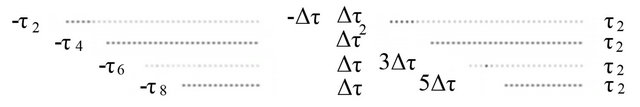 (b)
(b)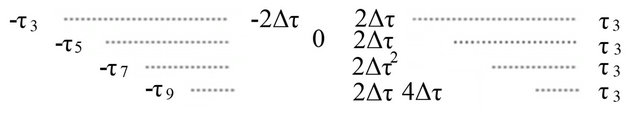 (c)
(c)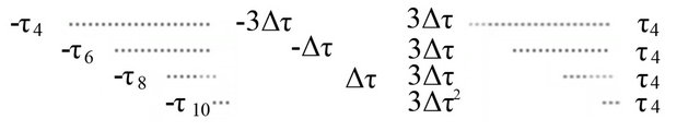 (d)
(d)
Figure 3. Time-shifted position of the peaks in the crosscorrelation between reference and other hydrophones; (a) Reference hydrophone S1; (b) Reference hydrophone S2; (c) Reference hydrophone S3; (d) Reference hydrophone S4.
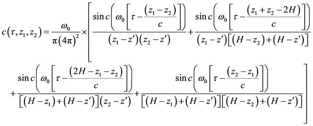
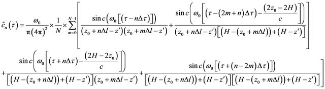
pair of hydrophones take part in the resultant cross-correlation function. The time domain cross-correlation function between signals received at two vertically separated sensors is given by [1,2,10] (see Equation (1) below).
where  is the bandwidth of the noise field, c the propagation speed of the signal,
  the depth of the seabed,
 ![]() and
and  the depth of the two hydrophones respectively and
  the small vertical distance of the surface noise plane underneath the surface.
3.1.1. First Stage of Beam-Forming
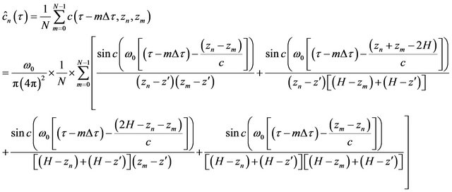
During the array processing for each reference hydrophone at depth,  , cross-correlation is performed with all other hydrophones at depth,
  in the array. Then all the correlation functions are averaged together after adjusting appropriate delay as described in section 2 so that a stronger correlation peak can be achieved. The average cross-correlation function [1] with respect to reference hydrophone at depth
  can be stated as
|
 (2)
(2)
where  is the propagation delay between two consecutive sensors.
All of the hydrophones in the vertical array are equally spaced, which leads to the following relationships
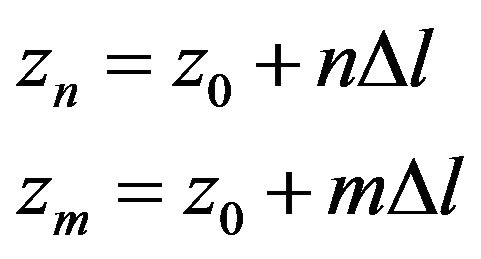 (3)
(3)
where  is the distance between two consecutive sensors and
 .
.
Substituting the value of  and
and  from expression (3), expression (2) can be re-written as
 (4)
(4)
Figure 6 shows the analytic plot of the correlation function after first stage of beam-forming considering the 4-hydrophone array. The parameters used in the analytic plot are  m,
m,  m,
m,  m,
m,  kHz,
kHz,  m/s and
 . A sampling rate of 90 kHz is used in the analytic plot, which gives 3 samples of spacing between two consecutive sensors.
Figure 6 shows that rightmost correlation peak moves towards the centre by 3 samples for the reference hydrophones  to
to  which shows the similarities with the conceptual diagram shown in Figure 4.
3.1.2. Second Stage of Beam-Forming
The average cross-correlation functions of first stage of beam-forming are combined again using DS beamforming to achieve much stronger correlation peak [1]. After the second stage of beam-forming, the cross-correlation function is given by
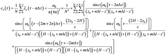 (5)
(5)
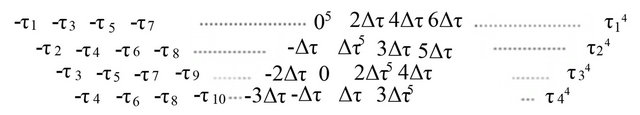
Figure 4. Position of the peaks of the average correlation function after first stage of beam-forming for all reference hydrophones.
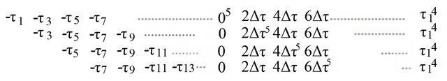
Figure 5. Position of the peaks of the time shifted correlation function in the second stage of beam-forming for all reference hydrophones.
 (a)
(a)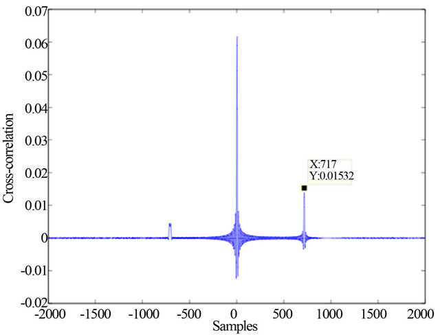 (b)
(b)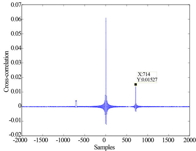 (c)
(c)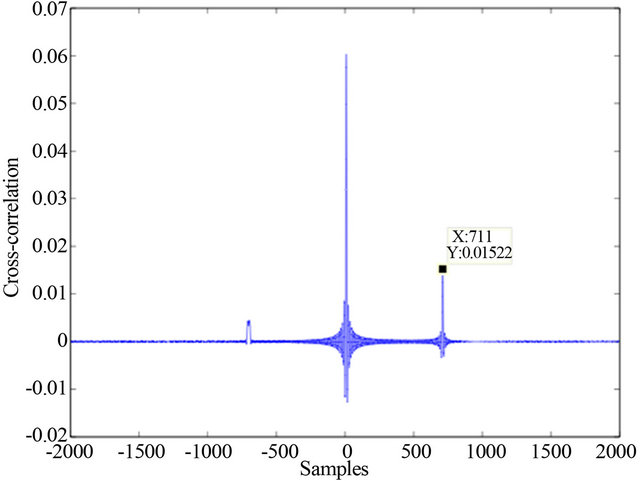 (d)
(d)
Figure 6. Analytic plot of the cross-correlation function of expression (4); (a) Reference hydrophone S1; (b) Reference hydrophone S2; (c) Reference hydrophone S3; (d) Reference hydrophone S4.
The third term of expression (5) shows that  numbers of the rightmost peaks coincide at
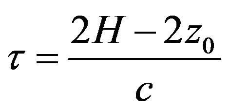
position. After averaging the strength of this peaks remains same as it was before beam-forming but the strength of correlation noise decreases because some of the correlation noises average out [1]. An analytic plot of expression (5) is shown in Figure 7 for the same parameters as Figure 6.
3.2. Power of the Correlation Peak and Noise
In the array processing, the resultant cross-correlation is the summation of  number of correlations in two beam-forming stages. Each correlation function between sensors
  and
and  consists of four sub-correlations considering the direct and first bottom reflected signals. This is because the cross-correlation between two sensors consists of the following four elementary cross-correlations 1) Cross-correlation between the direct paths of
  and
and .
.
2) Cross-correlation between the direct path of  and reflected path of
 .
.
3) Cross-correlation between the reflected path of  and direct path of
 .
.
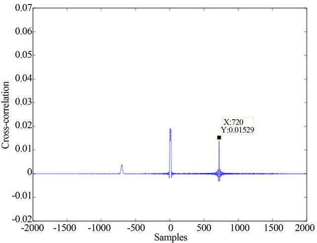
Figure 7. Analytic plot of the cross-correlation after second stage of beam-forming.
4) Cross-correlation between the reflected paths of  and
and .
.
The resultant correlation peak in the array processing is the summation of the correlation peaks that coincide with the peak of our interest in the beam-forming, with the resultant correlation noise being the combination of  number of elementary correlation noises. All of these noises are not independent because some of these noises fall on each other hence they are constructive rather than destructive. The following section describes how the resultant correlation noise and correlation peak are generated from elementary cross-correlation functions. The dependency of the elementary correlation noises on the final correlation noise is also described.
In Figure 5, each row from top to bottom shows the positions of the correlation peaks in the second stage of beam-forming for the reference hydrophones from top to bottom in the hydrophone chain. The peaks that coincide in the same point of Figure 5 create a group. Therefore, the elementary cross-correlation functions are divided into groups as follows
These 64 elementary cross-correlation functions are divided into twelve groups as shown in Figure 5. The correlation noise of each elementary correlation function inside a group fall on each other, hence they are additive. But the resultant correlation noises corresponding to different groups are independent relative to each other because different groups start at different positions. This results averaging out of the correlation noises of different groups, although their strength is different. Therefore, both the constructive and destructive effects of the elementary correlation noises affect the correlation noise of the overall cross-correlation process.
In this example, a 4-hydrophone array is used, but in general for a N-hydrophone array the total number of peaks are divided into groups as follows

To calculate the power of the correlation peak and correlation noise, attenuation needs to be considered for both the direct and reflected signals. The strength of the reflected signal is always less than that of direct signal because the reflected signal travels more distance compared to the direct signal. Since in the array processing hydrophones are very close to one another, it is assumed that distance between hydrophones are negligible compared to distance travelled by direct and reflected signal. If the power of the direct and reflected signals is attenuated by  and
and  respectively, the signals are attenuated by
  and
and ![]() respectively. Therefore the cross-correlation between direct signals and between reflected signals are attenuated by
respectively. Therefore the cross-correlation between direct signals and between reflected signals are attenuated by  and
and  respectively. Two other cross-correlations between direct and reflected signals are attenuated by
 . The variance of the resultant correlation noise considering attenuation is given by (see Equation (6) below)
where  is the variance of cross-correlation noise between hydrophones
  and
and , and
, and  the variance of the correlation noise after second stage of beam-forming. The variance
  can be expressed as [2,11]

where  is a constant which can be defined as the power spectral density (PSD) of correlation noise between hydrophones
  and
and . A total of 16 correlation peaks coincide at
 ![]() point for a 4-hydrophone array. For a N-hydrophone array,
point for a 4-hydrophone array. For a N-hydrophone array,  number of rightmost correlation peaks coincide at
 ![]() resulting a very strong correlation peak. The power of this rightmost correlation peak is given by
resulting a very strong correlation peak. The power of this rightmost correlation peak is given by
 (7)
(7)
|
where  is the power of a correlation peak of expression (5) which can be expressed as [2]
where  is a constant and can be calculated from expression (5).
3.3. SNR of the Cross-Correlation Function
In the passive fathometer application, SNR in the array processing technique is expressed as the ratio of the power of the emphasised correlation peak in the beamforming and the resultant correlation noise. From the expression (6) and (7), SNR is given by
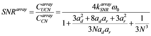 (8)
(8)
where the constant,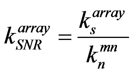 .
.
3.4. Resolution of the Cross-Correlation Function
Resolution of the cross-correlation function can be expressed as a function of the width of the correlation peak. The width of the correlation peaks only depends on the received signal bandwidth. So the two stages of beamforming in the array processing do not improve the resolution at all. In case of array processing resolution of cross-correlation function is directly proportional to the bandwidth of the noise field received by the array, which is fixed and given by [1,2,12]
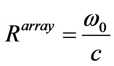 (9)
(9)
where  is the resolution of the correlation peak in the array processing.
4. Numerical Simulation
In the simulation, a 32-hydrophone vertical array is assumed to be placed at 4m depth in an oceanic environment where the depth of the seabed is 10 m. The separation between two consecutive hydrophones is 5 cm. A noise source is placed in the end-fire region of the array and a direct signal and a bottom reflected signal from the source come to all the hydrophones. The speed of the signal is 1500 m/s and the signals are being received by the hydrophones at a sampling rate of 90 kHz. The bandwidth of the acoustic noise signal is set at 15 kHz.
To compare the simulated results with the mathematics derived in Section 3, the simulation has been performed considering attenuation of the direct and reflected signals. At 15 kHz bandwidth, the spreading loss is the dominant source of attenuation [13]. Figure 8 shows the SNR of the cross-correlation function in the array processing.
The solid and the dotted lines of Figure 8 represent the simulated SNR and the analytic SNR respectively. The figure shows that simulation results are consistent with the mathematical results shown in expression (8). The only difference is that the simulated SNR is lowered by a constant term compared to the analytic result.
This is because, in theory it is assumed that a signal received by all the hydrophones are of same strength neglecting the inter hydrophone spacing. Therefore, the correlation noise  of expression (6) is constant for any combination of hydrophones
  and
and . However, in simulation, there is the difference of delays of a received signal at different hydrophones. The correlation noise
  in simulation is scaled by a constant term compared to
  in theory. Therefore the SNR in simulation is scaled by that constant term. This constant term can be estimated from the delay difference between hydrophones and signal source.
5. Comparison of Large Bandwidth and Array Processing Approach
The performance of the large bandwidth approach and the array processing approach will be evaluated in terms of SNR and resolution.
5.1. SNR Comparison
SNR of the large bandwidth approach is given by the following expression [2].
 (10)
(10)
where  is the SNR in the large bandwidth approach,
 ![]() the constant and B the bandwidth of the
the constant and B the bandwidth of the
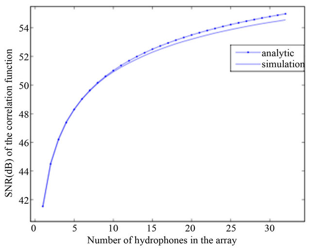
Figure 8. Analytic and simulated SNR of the cross-correlation function
noise field. The expression (10) does not consider attenuation in the direct and reflected signals. Considering attenuation in both the direct and reflected signals, SNR of the large bandwidth is given by
 (11)
(11)
where the direct and reflected signals are attenuated by  and
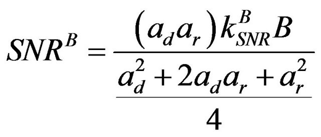
and  respectively. The SNR can be compared for the large bandwidth approach and the array processing approach from expression (11) and (8) as shown below
 (12)
(12)
where  and
and ![]() are the SNR constants in the array processing and the proposed technique respectively and they are about the same valued because these constants corresponds to the same correlation function in both the techniques. Expression (12) shows the following relationship between the two techniques.
are the SNR constants in the array processing and the proposed technique respectively and they are about the same valued because these constants corresponds to the same correlation function in both the techniques. Expression (12) shows the following relationship between the two techniques.
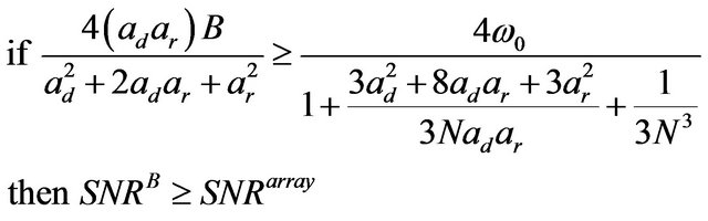 (13)
(13)
Expression (13) shows the SNR comparison between the two techniques, which gives the amount of bandwidth needed in the large bandwidth technique to achieve the same SNR with the N-hydrophone array.
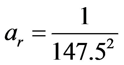
Let’s consider a practical scenario where a 32 elements array with 0.5 m inter-element spacing is used in the passive fathometry where depth of the seabed is 100 m. Most of the fathometer and bottom profile experiments use this type of array which has a design frequency of 1500 Hz. If the array is placed at about 52.5 m depth as it was the case in [1], the attenuation terms  and
and  of expression (13) can be expressed as
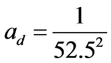
and
Only the spreading loss is considered in the attenuation, because this is the main source of attenuation up to a certain frequency neglecting absorption and dispersion loss. At 12.5 kHz, 50 kHz and 70 kHz absorption loss is about 1 dB/km, 10 dB/km and 20 dB/km respectively [13,14]. Therefore, in the application like passive fathometer, absorption can be negligible because the wind generated ocean surface noise is generally in the range of 100 Hz to 25 kHz and under the influence of rain it can be extended to 50 kHz [15-17]. Over 100 kHz absorptions are comparable with spreading loss and can not be negligible. Therefore, in the high frequency communications, active sonar and ultrasonic biological research, the absorption term need to be considered in the attenuation terms  and
and .
.
Using only the spreading loss in expression (13), a bandwidth of 5.4 kHz is required in the large bandwidth technique to achieve the same SNR as the array processing technique considering the design frequency of the array as 1.5 kHz. Anything beyond 5.4 kHz bandwidth in the large bandwidth technique gives further improvement of the SNR. The Figure 9 shows analytic plot of expression (13) which represents the comparison between the large bandwidth technique and the array processing technique in terms of SNR.
The comparison shown in Figure 9 considers that in the array processing a 32-hydrophone array of the design frequency of 1.5 kHz is deployed in a place where the depth of the seabed is about 100m and in the large bandwidth technique the bandwidth is being varied from 100 Hz to 50 kHz. The selection of bandwidth in the large bandwidth technique that gives the same SNR as the array processing technique depends on the number of hydrophones in the array, inter-hydrophone spacing and the attenuation of direct and reflected signals. The first two terms are dependant on array geometry which are fixed for a particular array and attenuation is dependant on the depth of the seabed.
5.2. Resolution Comparison
In the large bandwidth technique, we record a large band
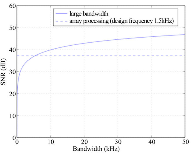
Figure 9. SNR comparison between the large bandwidth technique and the array processing technique where the bandwidth of the latter technique is 1.5 kHz.
signal compared to the array processing and in this case resolution is given by [2]
 (14)
(14)
where  is the resolution of the correlation peak and B the bandwidth of the noise field in the large bandwidth technique.
Comparing expression (9) and (14), the relationship between the resolutions of the two approaches can be expressed as
 (15)
(15)
Therefore, resolution is much better in the large bandwidth technique because in this technique, the bandwidth can be increased accordingly to achieve a desired resolution. But in the array processing technique, bandwidth is limited by consecutive sensors separation.
6. Conclusion
In this paper, it is shown theoretically that the large bandwidth technique gives better SNR and resolution of the NCF compared to the array processing technique upon satisfying certain conditions. The conditions say that the former technique gives better resolution if its bandwidth is just greater than the latter and improved SNR if its bandwidth is greater than the latter by a factor which is a function of bandwidth, number of array elements and attenuation. The improvement of SNR and resolution of NCF helps in the better estimation of the depth of the seabed. This is because the correlation peak becomes stronger and narrower with the increase of SNR and resolution. Therefore, the large bandwidth technique enhances the estimation of the passive fathometer using only two hydrophones compared to the array processing technique. One of the constraints of the large bandwidth technique is that it needs directional reception of the ambient noise from the end-fire region which is not a necessary condition in the array processing technique.
REFERENCES
- M. Siderius, C. H. Harrison and M. B. Porter, “A Passive Fathometer Technique for Imaging Seabed Layering Using Ambient Noise,” Journal of the Acoustical Society of America, Vol. 120, No. 3, 2006, pp. 1315-1323. doi:10.1121/1.2227371
- Md. Jahangir Alam, E. H. Huntington and M. R. Frater, “Improving Resolution and Snr of Correlation Function with the Increase in Bandwidth of Recorded Noise Fields during Estimation of Bottom Profile of Ocean,” Sydney, Australia, 2010.
- C. H. Harrison and D. G. Simons, “Geoacoustic Inversion of Ambient Noise: A Simple Method,” Journal of the Acoustical Society of America, Vol. 112, No. 4, 2002, pp. 1377-1389. doi:10.1121/1.1506365
- S. E. Fried, W. A. Kuperman, K. G. Sabra and P. Roux, “Extracting the Local Greens Function on a Horizontal Array from Ambient Ocean Noise,” Journal of the Acoustical Society of America, Vol. 124, No. 4, 2008, pp. 183- 188. doi:10.1121/1.2960937
- K. G. Sabra, P. Roux and W. A. Kuperman, “Emergence Rate of the Time-Domain Greens Function from the Ambient Noise Cross-Correlation Function,” Journal of the Acoustical Society of America, Vol. 118, No. 6, 2005, pp. pp. 3524-3531. doi:10.1121/1.2109059
- K. G. Sabra, P. Roux and W. A. Kuperman, “ArrivalTime Structure of the Time-Averaged Ambient Noise Cross-Correlation Function in an Oceanic Waveguide,” Journal of the Acoustical Society of America, Vol. 117, No. 1, 2005, pp. 164-174. doi:10.1121/1.1835507
- P. Roux, K. Sabra, W. Kuperman and A. Roux, “Ambient Noise Cross-Correlation in Free Space: Theoretical Approach,” Journal of the Acoustical Society of America, Vol. 117, No. 1, pp. 79-84. doi:10.1121/1.1830673
- M. Hawkes and A. Nehorai, “Acoustic Vector-Sensor Correlations in Ambient Noise,” IEEE Journal of Oceanic Engineering, Vol. 26, No. 3, 2001, pp. 337-347. doi:10.1109/48.946508
- K. G. Sabra, P. Roux, A. M. Thode, G. L. DSpain, W. S. Hodgkiss and W. A. Kuperman, “Using Ocean Ambient Noise for Array Self Localization and Self-Synchronization,” IEEE Journal of Oceanic Engineering, Vol. 30, No. 2, 2005, pp. 338-347. doi:10.1109/JOE.2005.850908
- F. B. Jensen, W. A. Kuperman, M. B. Porter and H. Schmidt, “Computational Ocean Acoustics,” American Institute of Physics, New Work, 1994.
- R. Pallas-Areny and J. G. Webster, “Analog Signal Processing,” Wiley-IEEE, New Delhi, 1999.
- S. A. Albahrani, M. R. Frater and E. H. Huntington, “Linearly Filtered Estimation of the Time-Domain Greens Function from Measurements of Ambient Noise,” Journal of the Acoustical Society of America, Vol. 124, No. 5, 2008, pp. 2699-2701. doi:10.1121/1.2981049
- J. Heidemann, W. Ye, J. Wills, A. Syed and Y. Li, “Research Challenges and Applications for Underwater Sensor Networking,” WCNC, 2006.
- H. Ochi, Y. Watanabe and T. Shimura, “Measurement of Absorption Loss at 80 khz Band for Wideband Underwater Acoustic Communication,” Japanese Journal of Applied Physics, Vol. 47, No. 5, 2008, pp. 4366-4368. doi:10.1143/JJAP.47.4366
- G. M. Wenz, “Acoustic Ambient Noise in the Ocean: Spectra and Sources,” Journal of the Acoustical Society of America, Vol. 34, No. 12, 1962, pp. 1936-1956. doi:10.1121/1.1909155
- D. H. Cato and M. J. Bell, “Ultrasonic Ambient Noise in Australian Shallow Water at Frequencies up to 200 khz,” Technical Report, DSTO Materials Research Laboratory, Urbana, 1992.
- L. Jianheng and G. Tianfu, “Model of Wind-Generated Ambient Noise in Stratified Shallow Water,” Chinese Journal of Oceanology and Limnology, Vol. 23, No. 2, 2005, pp. 144-151. doi:10.1007/BF02894230