ABSTRACT

In a multi-prize contest, we consider the space of all outcomes and define a probability on it by hypothesizing the probability of an outcome to depend on resources expended by all the players. In this probability space, we then derive the probability of an individual player winning. It turns out that this probability is a generalized Berry (1993) probability function. Specifically, when 0 weight is attached to the resources spent by the “unsuccessful players” (losers), the probability of winning of an individual player is proposed exactly by Berry (1993). Such a formulation also helps to alleviate charges against the probability function of Berry levied by Clark and Riis (1996) in the context of sequential distribution of prizes since prizes by our very hypothesis, are awarded simultaneously.

1. Introduction

Berry [1] analyses a rent-seeking model with multiple prizes/winners. By doing so, he generalizes Tullock’s contest success function (the technology or function that translates a player’s expended resources into his probability of winning) for one prize to the probability of winning in a multi-prize situation. If there are n players and k (denoted as in this note) many prizes, then Berry postulates that “the probability that firms ‘n’ wins is dependent upon its rent-seeking expenditures in combination with the expenditures of all other possible combinations of ‘’ firms (out of ‘n’ firms) divided by the combinations of all possible ‘k’ firms’ expenditures.” (p. 438).

The main gap in Berry’s analysis is that it starts directly by postulating the probability of an “event” (that a player wins a prize) without specifying the set of “outcomes” (where an outcome means the distribution of the limited number of prizes among the competing players. See section II for a mathematical definition) and the corresponding probabilities, which is necessary for a mathematical formulation of the problem. Clark and Riis [2] criticize the ad hoc-ness of Berry’s approach from a different perspective (see below) and they also miss to lay down the underlying probability space of Berry’s model. This paper resolves this issue completely and proposes a concrete probabilistic foundation of Berry’s approach.

Clark and Riis [2] note that Berry’s probability of winning function is a valid probability function (though not deriving it from the underlying probability space) but they criticize it on the ground that it implies an “unreasonable selection process” of the winners in which “rentseeking outlays affect only the distribution of the first prize; after this is awarded, rent-seeking outlays are forgotten and each player has an equal probability of winning” (p. 179). But their criticism holds only when the process perceived is one where the announcement of outlays by the players is simultaneous while the distribution of prizes is sequential (like the distribution of quotas by the government, or the promotion of several workers. See Clark and Riis [3]).

However, often the process in contests can be perceived to be one of not only simultaneous announcements of efforts but also simultaneous distribution of prizes. Examples include occupying seats in a congested transport vehicle by passengers, getting admitted to limited number of seats in elite educational institutions, or getting housing allotments in the regulated housing market. (Keeping these examples in mind, we use the terms “resources”, “expenditures” and “efforts” interchangeably, in the sense of outlays expended by the players participating in the contest.) Our probability space, by the very way it is defined, is more amenable to model such simultaneous distribution of prizes and since we can derive Berry’s formulation from it, our model can dispel Clark and Riis’ criticism leveled against it (see especially footnote 1).

We start from the space of all possible outcomes and make the following plausible hypothesis: let the probability of an outcome depend on the (weighted) sum of efforts of all the players. In the resulting probability space, we derive the probability of success (winning a prize) for an individual player (which is in contrast to both Berry [1] and Cark and Riis [2], who start from the probability of winning of individual players).

We find that if the efforts of the unsuccessful players are weighed equally like those of the successful players, then we end up with an equal probability model where each player has an equal chance of winning, irrespective of their expended resources. On the other hand, if the resources expended by the unsuccessful players receive no weight at all (that is 0 weight) in bringing about a realized outcome (that is the probability of the outcome depends only on the resources expended by the successful players), then the resulting probability of winning of an individual player turns out exactly to be Berry’s formulation. Thus, in particular, our model generalizes Berry’s probability function.

The next section begins from the probability space and derives a probability function by postulating a plausible hypothesis (Assumption 1) for the probability of outcomes, and demonstrates that Berry’s formula can be derived from it as a special case.

2. The Model

Let there be n players and, many prizes. The set of all possible outcomes can be represented by the collection of vectors

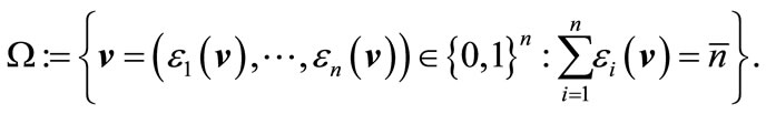(1)

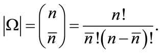
here means that in the outcome the i-th person is successful in winning a prize, and otherwise. The restriction reflects the fact that in any outcome all prizes are taken. Also note that the number of different outcomes¹ in the space is given by

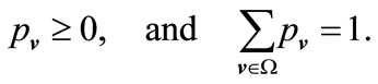
A probability on the space is given by a collection of non-negative real numbers allotted to each outcomes, satisfying the two conditions

The pair is said to form a probability space.

The question we are asking is the following: Can we have a probability space (on the sample space given above) such that the probability of any outcome reflects the collective effort of the mode of the outcome (the way the outcome comes about)? To answer the question, let us hypothesize the following:

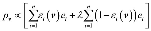
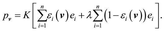
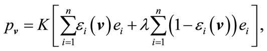
Assumption 1. Let probability be proportional to the weighted sum of the efforts of all the competing players. That is,

(2)

where be the effort exerted by the th player to obtain a prize out of available units, with, , and is the weight attached to the efforts of the players who are not successful in winning any prize.

This assumption means that there exists a positive constant (not depending on the outcome) such that

The following proposition lays down the value of, the probability of an outcome, , and the probability of “success” for player i,:

Proposition 1. Consider the probability space given by (1). Then, under Assumption (1), the probability of outcome is given by

(3)

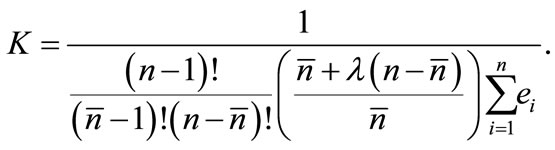
where the constant of proportionality is given by

(4)

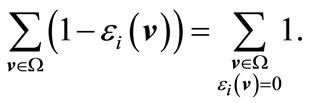
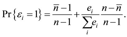
Moreover, the probability of success for player i is:

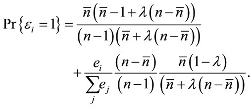(5)

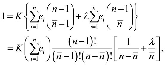
Proof. Derivation of K: The derivation of the constant of proportionality K is as follows: The non-negativity of just means that K has to be non-negative (as the efforts). The second criterion is satisfied if and only if

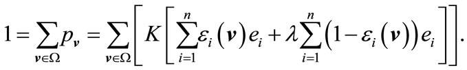
Since K is an absolute constant and not depending i or we can take it out of the summations to get

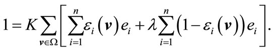
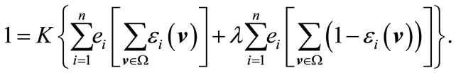
Next we interchange the order of summations

In the inner sum, since the effort does not depend on (this is by assumption, since we do not allow different efforts for different outcomes), we can take it out to get

Now consider the inner sums over. Here,

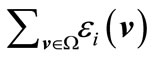is just the count for the number of outcomes for which. That is,

From simple combinatorics, we get that this count is same as the number of vectors of length, with 0, 1 entries such that entries have value 1 and others have value 0. This is given by Similarly, is just the count for the number of outcomes for which (since otherwise the contribution is 0). That is,

From simple combinatorics, we get that this count is same as the number of vectors of length, with 0, 1 entries such that entries have value 1 and others have value 0. This is given by. Substituting we get the following calculations

Hence,

Substituting we can get. This completes the derivation of the probability space in the case of our model. Now we come to the next part of the proposition.

Derivation of individual’s probability of success: Consider person 1. Let us compute the probability that person 1 is successful using the above probability model:

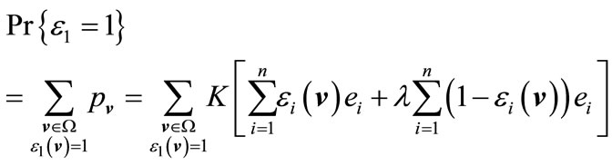
where K is as given by (4)

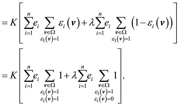
Now

and

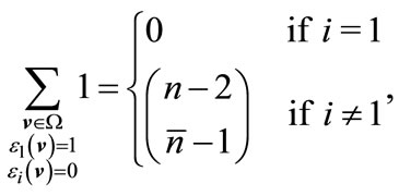
Substituting and simplifying, we get

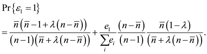
Substituting subscript 1 with i, we can get (5). This completes the proof.

Notice that in this model, if, we see that the probability of any outcome depends on the efforts of the people who are successful only, while means the probability of any outcome depends equally on the efforts of those who are successful as well as those who are not so. For any, it means the efforts of those who are successful contribute more towards bringing about the outcome than the efforts of those who remain unsuccessful.

Notice the following easily derivable properties of our model. If, we get

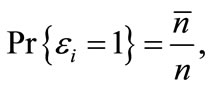
which is the equal probability model. This means that if people’s efforts are equally weighted in the probability of an outcome, irrespective of whether they are ultimately successful or not, then each individual has the same probability of being successful, irrespective of effort levels.

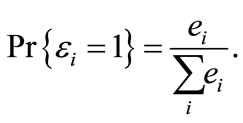
Derivation of Berry’s probability function: Note if, we get

(6)

This is the same expression as introduced by Berry [1] and also rearranged and reproduced in Clark and Riis [2]. (An example of the above probability model can be found in Appendix A.) As noted by Berry [1], in case of a single prize, the probability of success of the ith individual reduces to the classic Tullock’s contest success function (obtained by substituting in (6)), given by

(7)

The probability function also exhibits the usual properties (as also noted in Clark and Riis [2] and (1998)) in that it is bounded between 0 and 1, the probability of winning of a particular player is increasing in one’s own resources, decreasing in other’s resources, and the sum of all players’ probability of winning one of the prizes equals, the number of prizes.

An interpretation for: Suppose we are interested in the finding out how the probability of being successful changes as the weight given to efforts of people who are unsuccessful, , changes². That is, we calculate as follows:

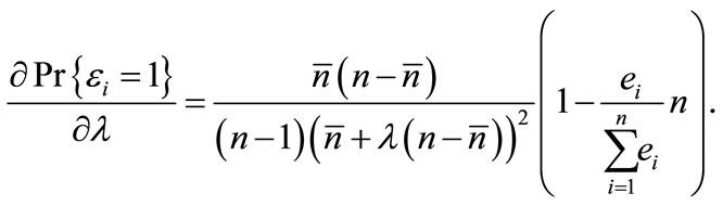
Hence the probability increases or decreases with, depending on individual effort e_i, relative to the average. In particular, if, that is , then. (Similarly, if , the opposite holds.) This means that if individual i is exerting less than average effort, then as desired, his probability of success falls, as falls. Similarly, for someone exerting more than the average effort, the above derivative is negative, which means that his probability of success increases as falls.

The last observation means that in our probability model, the smaller gets, the more the probability of success of someone who is exerting above average effort, and lesser is the probability of success of someone who is exerting less than average effort. In the extreme case we have which means the probability of an outcome is sensitive only to the efforts of those who have succeeded. Hence makes for a good case to work with, which again means that our probability of success turns out to be that of Berry’s.

3. Conclusion

In this note, we derive a probability function by hypothesizing a possible relation between outcomes and efforts/resources of players in the context of a multi-prize contest. When efforts are simultaneously exerted by players, multiple prizes are simultaneously awarded, we hypothesize that the probability of an outcome is proportional to all efforts exerted. In the special case, where the probability of an outcome is proportional to the effort exerted by the winners only (that is to say the weight attached to the efforts of the unsuccessful players is 0), the probability of an individual player winning is proposed exactly by Berry [1]. Hence we provide a probabilistic foundation for the probability function in a multi-prize rent-seeking contest as introduced by Berry. Moreover our probability model, by the very way it is defined, is a good depiction when prizes are simultaneously distributed.

REFERENCES

Appendix

Derivation of the Probability Model with an Example

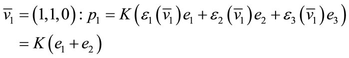
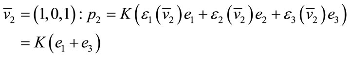
Consider the basic probability model with (which gives Berry’s probability function). Let,,. Then the possible outcomes and associated probabilities are as follows:

Hence summing over all outcomes we get,

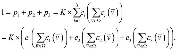
Now:

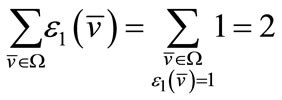
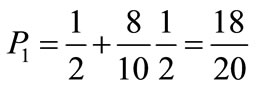
and similarly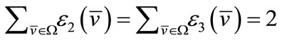. Hence substituting we get

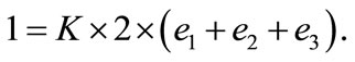
And, for this example.

Now consider an example with, , ,. Then we get the following:

Again the sum equals. This means (roughly) that person 1 exerting high effort gets to win a prize with a very high probability, while the other two players exerting the same low probability gets to win the remaining prize with almost equal probability.

NOTES

¹Note that in any particular outcome, we have many one’s and many zeroes in a certain order, but the one’s (or the zeroes) are unordered among themselves. Hence the situation depicts prizes awarded simultaneously. In contrast, if we had sequential distribution of prizes, then the set of outcomes would be given by

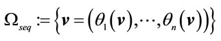
where means the i-th player is unsuccessful whereas means the i-th player has won the j-th prize, , in the outcome. That is, is the set of all possible permutations of.

²Notice that in our probability model, the space is essentially given by a collection of non-negative real numbers allotted to each outcomes, satisfying the two conditions

Hence for every, the pair is said to form a probability space. Now here we want to see if we can choose a particular (and hence the corresponding probability space) to work with.

REFERENCES

- S. K. Berry, “Rent-seeking with Multiple Winners,” Public Choice, Vol. 77, No. 2, 1993, pp. 437-443. doi:10.1007/BF01047881
- D. J. Clark and C. Riis, “A Multi-Winner Nested RentSeeking Contest,” Public Choice, Vol. 87, No. 1-2, 1996, pp. 177-184.doi:10.1007/BF00151735
- D. J. Clark and C. Riis, “Influence and the discretionary allocation of several prizes,” European Journal of Political Economy, Vol. 14, No. 4, 1998, pp. 605-625. doi:10.1016/S0176-2680(98)00028-7