Journal of Mathematical Finance
Vol.07 No.03(2017), Article ID:77621,26 pages
10.4236/jmf.2017.73030
Nonparametric Model Calibration for Derivatives
Frédéric Abergel, Rémy Tachet des Combes, Riadh Zaatour
Laboratory MICS, Centrale Supélec, Châtenay Malabry, France

Copyright © 2017 by authors and Scientific Research Publishing Inc.
This work is licensed under the Creative Commons Attribution International License (CC BY 4.0).
http://creativecommons.org/licenses/by/4.0/


Received: April 26, 2017; Accepted: July 10, 2017; Published: July 13, 2017
ABSTRACT
Consistently fitting vanilla option surface is an important issue in derivative modelling. In this paper, we consider three different models: local and stochastic volatility, local correlation, hybrid local volatility with stochastic rates, and address their exact, nonparametric calibration. This calibration process requires solving a nonlinear partial integro-differential equation. A modified alternating direction implicit algorithm is used, and its theoretical and numerical analysis is performed.
Keywords:
Local Stochastic Volatility, Calibration, Derivative Pricing, Partial Integro-Differential Equations

1. Introduction
One of the most important challenge for real-life applications of a model to derivatives trading is the issue of calibration. Similar to common situations in many areas of physics and engineering, once a model has been suggested, its parameters have to be estimated using external data. In the case of derivative modelling, those data are the liquid (tradable) options, generally called vanilla products.
It is well-known since the pioneering work of [1] and its celebrated extension by [2] that the knowledge of market data such as the prices of vanilla options across all strikes and maturities is equivalent to the knowledge of the risk-neutral marginals of the underlying stock distribution. Here, we are interested in appli- cations of this result to three different cases.
The first one is quite classic, and is the starting point of our work: local and stochastic volatility models. Such models are very useful in practice, since they offer both the flexibility and realistic dynamics of stochastic volatility, and the exact calibration properties of local volatility. The problem of calibrating local and stochastic volatility models has been dealt with for a while now, for instance by [3] . However, practitioners seem to agree that the stability of its resolution becomes uncertain when the volatility’s volatility is too large. We shall see that indeed some kind of instability appears, and offer explanations to the phenome- non. The second case we focus on is the correlation between assets. Empirical measures give a certain set of results. However, when modelling a basket on multiple underlyings, a problem occurs. If one uses local volatility models for each underlying and correlates their brownian motions using the empirical correlation, the basket obtained will not reproduce the vanillas quoted on the market. This raises significant issues when hedging products on multiple under- lyings. One of the solution for this problem is the known ‘local correlation’ approach: the correlation matrix for the n underlyings is deformed using a parameter, function of the time and the basket level. Here, we use that approach to obtain a calibration equation for the basket, relatively similar to the one appearing in the local and stochastic volatility model, and then numerically solve said equation in a two-underlyings framework.
The last topic we shall be interested in are interest rates, we study a hybrid model: local volatility with stochastic rates. Using a partial differential equation approach similar to the local correlation and the local and stochastic volatility, we write a calibration equation for the vanillas of this hybrid model, solve it and verify the accuracy of the fit.
The general form of our calibration equations is nonlinear partial and integro- differential. For their resolution, we chose to adapt the alternating direction implicit scheme (very efficient to solve classic linear second order parabolic equations, [4] ). Being in a nonlinear non-local framework, many questions arise. Is it relevant to use ADI algorithms to solve the equations stemming from our calibration problems? How should we deal with the nonlocal term? Is the finite difference scheme we chose consistent, and what is the order of the truncation error? Can we detect an instability in certain cases? Is it possible to explain it?
The aim of this work is to address and at least partially answer these questions. The paper is organized as follows. In Section 2, we quickly present the case of the local and stochastic volatility model. Section 3 is devoted to the local correlation, its calibration equation and the fit we obtain in the case of a basket on two underlyings. In Section 4, we do the same thing in the stochastic rates frame. Finally, in Sections 5 and 6, we adress the questions raised previously concerning the ADI algorithm used for the resolution, Section 7 is a brief conclusion.
2. Local and Stochastic Volatility Models
2.1. Partial Integro-Differential Equation for the Calibration of LSV Models
The diffusion model is assumed to be the following
(1)
(2)
is the stock price process and the stochastic component of the volatility. The function b simply transforms that factor into a proper volatility. a is the local volatility part of the model, exactly as in Dupire’s formula, its value shall be specified depending on the aimed vanillas. is the volatility of the volatility factor (commonly called “vovol”) and is a drift term. and are one-dimensional standard brownian motions with correlation .
Let us now consider a surface of vanilla prices and the corres- ponding Local Volatility . Under suitable regularity and ellipticity assum- ptions, the following proposition can be proved
Proposition 1. The diffusion model defined by (1-2) has a density with respect to Lebesgue’s measure. Moreover, if the model fits the surface of vanillas then necessarily
(3)
Proof. The exact assumptions and the existence proof can be found in [5] . Here, the main concern is the calibration result. Let us assume that the model fits exactly the surface C. Letting denote the initial state of the system, the joint density of the couple verifies Kolmogorov for- ward equation
Applying Fubini, let be the first marginal density of our couple. It is possible to integrate the previous equation and obtain
In the case of a local volatility model ( and ), the density of the Spot process solves the equation
The vanillas of the LSV model being perfectly fitted, we have . Iden- tifying the terms in the two last formulas gives
Using this proposition, and reintroducing the value of a in Kolmogorov forward equation, the joint density is then solution of the nonlinear partial integro-differential equation
(4)
(5)
There is thus equivalence between the existence of a model (1-2) that calibra- tes the vanillas C and the existence of a solution p to the pide (4).
Remark 2.1. The quotient is nothing but the conditional expecta-
tion of the volatility squared, knowing the spot process. This result is not original in itself (by applying the theorem from [6] for instance), the partial differential equation method however is unusual, and will be used on the other models as well.
The theoretical study of Equations (4) and (5) can be found in [7] . Existence of solutions is proved under strong assumptions (especially on b, which must be sufficiently close to a constant). The general resolution remains an open pro- blem.
2.2. Numerical Results
It seems to be well-known among practitioners, that instabilities occur in their calibration when the volatility’s volatility (in the notations, function ) is too large. This seems to confirm the theoretical limitations met trying to prove the global existence of a solution: when the function b oscillates too much (a change of scale in the factor clearly shows the equivalence between a b that moves a lot and a large ), the resolution of the equation is not guaranteed anymore. To assess these statements, we considered our problem from a practical viewpoint.
In this section, the calibration that stems from solving the partial differential Equation (4) is studied, for two stochastic volatility models: a lognormal one and a “Cox-Ingersoll-Ross” process. The details of the algorithm used for the resolu- tion and a study of the instabilities will be treated later, in Sections 5 and 6.
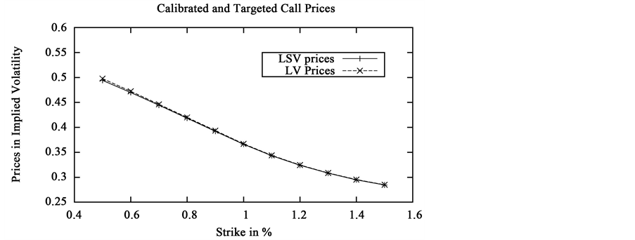
2.2.1. Lognormal Volatility
Starting with a simple mean reverting model for the volatility factor, the func- tion b is chosen as an exponential
(6)
(7)
with
Equation (4) is solved using the functions we just chose and the local volatility associated to the EuroSTOXX 50 implied volatility surface of 2009/04/02. Once function p, density of the couple , is found, we compute the vanilla prices for different strikes and maturities using this density. To have a point of comparison, the same prices are also computed with the local volatility , both of them are then compared to the targeted prices (column TP).

Let us then plot the error between the original vanillas and the ones obtained with the model. The calibration is quite efficient, the errors are equivalent to the ones of the local volatility model.
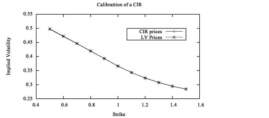
2.2.2. Cox-Ingersoll-Ross Process
We also focus on the calibration of a model inspired from the interest rates framework: the volatility is assumed to follow a CIR process.
(8)
(9)
Detailled properties of this process are described by [8] . In particular, as long as , is strictly positive a.e. Once again, Equation (4) is solved with this stochastic volatility.
3. Application to the “Local Correlation” Model
In this chapter, we are interested in the calibration of a market with n stocks and a basket on those stocks. The purpose is to define a diffusion model for those underlyings that is able to reproduce their implied volatility surface as well as the one of the basket.
The notations are the following, let denote the n stocks involved in our problem. The basket's value is given by
(10)
where the set stands for the weights of the different underlyings. They are assumed to be constant in the rest of our work. Let us also fix surfaces of vanillas and .
3.1. Inconsistencies between Stock and Basket Options
The naive approach to solve this problem is simply to consider n local volatility models
(11)
The functions are easily determined to fit the surfaces with this diffusion. The correlation matrix associated to the standard brownian motions of each underlying can be estimated with historical data. The model is now entirely defined. By Equation (10) of , the vanilla prices for the basket are completely determined and are equal to
. However, there is no particular reason for the surface
computed in this framework to be equal to . In fact, the skew of the basket is more pronounced on the market than in a model with constant correlations between the underlyings, [9] .
3.2. “Local Correlation” Model
In the manner of B. Dupire who decided to let the volatility depend on the level of the spot process, a degree of freedom is added to our model by distorting the matrix of correlation with a function of . This method appears for instance in [5] [10] where the basket level induces some feedback on the values of the different underlyings. In our context, the new correlation matrix is taken as a linear combination of and the constant matrix with only 1 as coefficients. This matrix is equal to
(12)
We shall see while writing the calibration equation that has to be chosen as a function of the time and of . The matrix can be seen as an analo- gous of Dupire's local volatility, a 'Local Correlation' so to speak. Assuming that is a proper correlation matrix (definite, positive...), and that the coefficients of the diffusion have a sufficient regularity, our diffusion model then possesses a density in the more general case of a matrix function of the couple . It is also possible to write a condition for the vanillas of the model to be fitted.
Proposition 2. The diffusion model defined by (11) with a correlation function of the couple , has a density with respect to Lebesgue's measure. Furthermore, this model calibrates the surface of 's vanillas (represented by its local volatility surface ) if and only if
(13)
where
with
(14)
Proof. The existence of the transition density stems from the assumptions made on the regularity of the coefficients, and on , for more details see [5] . We can now write the calibration problem for the vanillas of the basket . The density just defined satisfies Kolmogorov forward equation
To ease the problem, it is useful to change the coordinates into with defined by (14). After computations, the equation be- comes
where and are defined above. Integrating the equation against the variables , and writing , the density of the marginal law of B satisfies
Comparing this equation to Dupire’s equation for the local volatility
if our model reproduces the vanillas , then the following equality must be verified
Reciprocally, the condition we just wrote is clearly sufficient for the options to be calibrated
Remark 3.1. Let us note that this condition is written as an equality between two functions of the time and of B. The other variables are no longer repre- sented.
Assuming that condition (13) is not verified, the model defined by (11) does not fit the vanillas of the basket . It has to be enriched to solve the calibration problem. Our choice is to distort the correlation matrix. The new matrix is described by (12). Hence, let denote the matrix for all . We also notice that, the trace of being equal to n, its smallest eigenvalue is smaller than 1.
Lemma 1. The matrix is also a correlation matrix as long as is in with
(15)
Proof. Clearly, for all
If is positive, since is stricty positive, the matrix remains definite positive. Now, if , Cauchy-Schwarz gives
Since , is enough for to be stricly po- sitive.
The diagonal coefficients of are still 1. As for the other terms, thanks to the first term in relation (15), they still belong to the interval .
We introduce the new correlation matrix in condition (13), this gives
(16)
is a function of B and t. It is now possible to use this value to write a pide on the density . Any solution of the following equation is a density that calibrates the vanillas of the basket
(17)
where is linear and verifies
and is the nonlinear part of the equation
Remark 3.2. The operator stems from a change of coordinates on a uniformly elliptic operator. It is also elliptic, uniformly on any domain where the are bounded away from 0 by a strictly positive constant.
Furthermore, the initial condition is
where is the market value at instant 0 of the i-th stock. Applying this initial condition to (16), the initial value of is equal to
(18)
For a theoretical study of the calibration equation, we refer the reader to [5] .
3.3. Resolution of the Equation for the Calibration of a Basket
This subsection focuses on the results of the calibration for a two-underlyings basket. Let us consider two assets, both of them are assumed to generate the following implied volatility surface.
Using a Monte-Carlo simulation and the local volatilities stemming from those surfaces, the theoretical prices for the basket are computed, with weights and a correlation .
Distorting this theoretical surface by a factor of 0.9, and thus making the prices of the basket inconsistent with the prices of the underlyings, the calibration algorithm is applied. Solving the partial integro-differential Equation (17) gives the following vanillas (quoted in implied volatility).
Here are some results for other tests. We calibrate a model with the following parameters , and , the targeted surface is the theo- retical one distorted with two factors: first 0.95 and second 1.05.
At last, a different surface for the second underlying is chosen, mutliplying the first one (described in 3.3) by 0.9, the correlation is this time taken as 0.5.
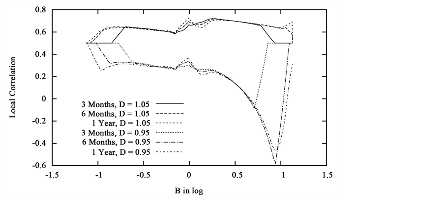
The results are rather satisfactory, especially at the money. To keep the computations to a reasonnable duration, a sparse initial surface was used. This explains why the calibration is not better far from the money, the fitting method is nontheless valid. Now follows an outlook of the values taken by the new correlation at different maturities when the theoretical surface is distorted by factors 0.95 and 1.05. The parameters are: , and .
As expected, the Local Correlation and the distorsion factor evolve in the same direction. The underlyings must be more correlated when the implied volatility of the basket is higher, and reciprocally. Furthermore, it appears that in the case of the 0.95 distorsion, the correlation has to violently decrease for high values of B: the two underlyings must be anti-correlated when they are both large.
As for the influence of the maturity, let us first state that in the computation of , when the denominator is smaller than , we chose not to change the correlation, to avoid numerical errors. It appears that, as long as B is in a zone where was actually computed, the framework chosen to test the calibration actually generates a local correlation constant in time.
4. Application to Stochastic Interest Rates
This section is dedicated to hybrid local volatility models with stochastic rates. The interest rate is assumed to be stochastic and to follow a diffusion equation. The volatility depends on the level of the spot process exactly as in a local volatility model. The idea is to compute its exact value for the vanillas in this model to be calibrated.
4.1. Calibration of the Hybrid Local Volatility Model
The risk-neutral diffusion of the model is written as
(19)
The two brownian motions are correlated with a constant correlation denoted by . Classic regularity and ellipticity assumptions are made on the coefficients of the diffusion (described in [5] ) to get the
Proposition 3 The diffusion model defined above has a transition density with respect to Lebesgue’s measure. The value of that fits its vanillas is given by
(20)
where is the density of the couple , and a determini- stic curve of rates used in the computation of Dupire’s local volatility .
Proof. The existence of the density stems from the assumptions on the coefficients. Let us prove formula (20). The function p solves the forward parabolic equation
with the initial condition . As previously, the equation is inte- grated with respect to y, writing
This equation needs to be matched with
Both of them can be written as
Computing
where the second line stems from a simple integration by parts. Reintroducing this into the previous equations, we get
In order to calibrate the vanillas, all that remains to be done is match the marginal density q with , giving the necessary condition
Replacing q by completes the proof.
The calibration equation for the vanillas of our hybrid model is thus
(21)
with given by Formula (20). Using similar technics to the other cases, an existence result can be obtained under certain assumptions, but this is not the scope of this paper. It is however noteworthy that one of the necessary hypothesis is the small variation of function r with respect to the deterministic curve .
4.2. Numerical Calibration
In this section, the theoretical results above are applied to calibrate a given diffusion model. Assuming the instantaneous rate to obey a Vasicek model (or in other words an Ornstein-Uhlenbeck process), the diffusion equations become
The ADI algorithm described in section 5 is applied to Equation (21) with the coefficients associated to this diffusion. The initial condition is .
As in the two previous sections, this partial integro-differential equation is solved with a variable change for the spot process . The grid chosen is with and . We discretize it with 300 points in both the spot and the rate direction. The initial condition (Dirac mass at the point ) is approximated by a bivariate Gaussian centred at that point with a very small variance.
The following numerical values are taken for the diffusion
These values generate the interest rate
To assess the quality of the calibration, call and put options on the spot process are computed by integration on the grid and compared to the targeted prices (target columns). Convergence is quite satisfactory. For instance, for 6 months and 1 year maturity vanillas, one finds
5. Algorithm for the Resolution of the Calibration Equation
In the previous sections, we wrote the calibration equations and gave graphs for their efficiency. In this one, we describe the algorithm used to solve them: a classic alternating direction implicit scheme. The nonlinear term is handled using a forward induction at first, and then a predictor-corrector method.
The strong feature of an ADI scheme is its convergence rate in time and space: . The nonlinearity of the equation challenges this assertion. It is however possible to prove that it remains true in this case too.
5.1. Alternating Direction Implicit Scheme
The calibration equation is a second-order parabolic equation. One of the most efficient method to solve such equations is a finite-difference approximation with alternating direction methods. For more informations on the subject, the reader can look into [4] , numerous articles have also been published, in particu- lar [11] [12] [13] [14] . Let us now consider the following equation
(22)
(23)
where f, g, , and are functions of t, x and y, a constant and the quotient of integrals
(24)
Remark 5.1 We restricted ourselves to two-dimensional equations since they cover all the concrete examples studied previously. But the computations that follow are true in the general case. The cost in time however becomes an issue in higher dimensions.
The domain for the numerical resolution is . The first step is to take care of the initial condition. Instead of the Dirac, the initial condition is chosen as a gaussian distribution with very small variance. It obviously approximates our initial condition. It also verifies (on any bounded domain) the properties of regularity and strict positivity required in the theoretical study of the Equation (though in the present section, we are only interested in its numerical resolution). Let if or be the boundary conditions.
The algorithm is based upon a predictor-corrector approach. Let , and be increments of the variables x, y and t, where , and with I, J and N integers. The sets of points in the x,y,t-plane is given by , and , for , and . We construct four sequences , , and of space-dependent functions with n between 0 and N.
A classic alternating direction implicit scheme functions as follows: let us define the initial functions
and then by induction
(25)
(26)
where designates (the same thing being true for the other coefficients of the equation). is a difference operator for the space derivatives. For instance, with and
The Equations (25) and (26) form two tridiagonal systems that can be solved very efficiently. A recursion formula can be computed on the functions defined above
Thus
And eventually
(27)
In the litterature concerning alternating direction implicit schemes, the functions are often called the predicted value of the solution p, a second “corrector” step usually follows. In our case, the equation being nonlinear, we start by chosing and study the finite-difference approximation that results.
Proposition 4. This last finite-difference equation is consistent with the partial differential Equation (22) on a bounded domain with smooth initial condition , the truncation error is
Proof. Let p be a classic solution of Equation (22) on a bounded domain, with . We assume that p is strictly positive and sufficiently differentiable for all the quantities in the sequel to be properly defined. All the derivatives that appear are bounded as a consequence of the regularity assumptions on p. Writing , a simple Taylor expansion with re- mainder gives
As for the space derivatives, clearly
where the different constants are between 0 and , or de- pending on the context, they may change from one formula to another. Let E denote the truncation error for Scheme (27), we have
Applying the previous expansions and using the fact that p verifies Equation (22) at times and gives us
with the error coming from the time-derivative
, and come from the second order space-derivatives
enables us to compensate for both the nondiagonal term and the nonlocal term that cannot be computed implicitely
and are the terms corresponding to the first order space-derivatives
At last, is the correction term stemming from the alternating direction implicit scheme
Thanks to the regularity of p and of the coefficients of (22), the upper bounds , , and are
obtained. It is also easily proven that . The term that prevents us from getting an error in is . All we have is . This concludes the proof.
Remark 5.2. In a case with no term, the equation is a classic linear and parabolic one. In that case, when the off-diagonal1 term is absent ( for instance), the previous scheme has an error in . To obtain such an error in the general case, a second “corrector” step is generally used: the predicted value is introduced as an approximation of in the cross-derivatives. Here, we use it in the nonlocal term too.
The correction step is the following
Here too, one can compute
Eventually, a Crank-Nicholson like formula appears
Let us study the consistency of this new scheme
Proposition 5. The algorithm with a corrector step is also consistent. The truncation error is
Proof. To prove the consistency, let be defined as
The computations are almost identical to the previous proposition. This time the error is equal to
Using the same decomposition, the errors , , and do not change. is slightly different but still in . As for and , we now have
which also verify and . The real difference can be seen in
The important feature of the predictor is that the difference is . This gives and concludes the proof.
5.2. Time Convergence Rate of the Modified ADI Algorithm
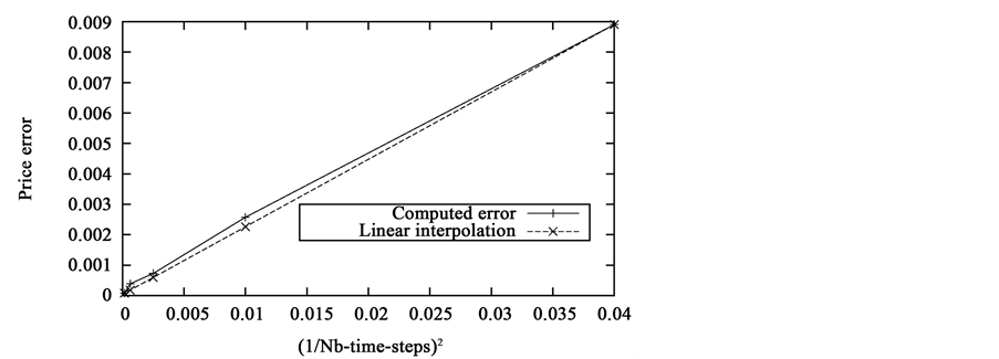
In this brief section, we compare the convergence of the algorithm with the theoretical rates computed in the previous part. To do so, the calibrated value of 1-year at-the-money vanillas is computed for different number N of time steps. We then plot the error between this price and the targeted value against N. The next graph is obtained with the one-step predictor algorithm.

The error is clearly in as was proved in Proposition 4. We conduct the same experiment with this time both the predictor and the corrector steps.
This time too, numerical experiments seem to agree with theory. The error appears to be in . The predictor/corrector scheme serves its purpose.
6. Instabilities of the Solutions: Numerical Explosion for “Oscillating” Volatilities
In the previous sections, we described the algorithm used to solve the different calibration equations concerned by our work, and also mentioned the theoretical research performed on the subject. Though a partial existence result for Equation (4) was found, it was still impossible to prove it in the general case: a strongly variable function b.
This last section is devoted to the local and stochastic volatility model, from that point of view. The numerical resolution of the calibration is performed for strongly variable functions b.
At first, let us go back to the equation for the calibration of a local and stochastic volatility model. For the sake of simplicity, the interest rate is assumed to be zero. The equation is the following
(28)
The existence of a solution to this Equation (on a bounded domain, with regularized boundary conditions) was previously stated under certain assump- tions on b, the essential one being: there exists a constant such that for a given . Using the algorithm described in the previous section, we are now interested in the behavior of the numerical solution of (28) when the function b violates the assumption.
The model chosen for this study is the mean-reverting volatility already expounded
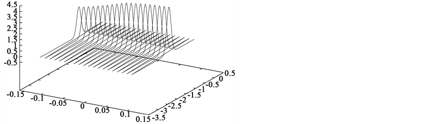
with , and three strictly positive constants. The values chosen in Section 2 for the different parameters of the model and of the algorithm led us to a satisfactory calibration. Using them once again, we plot on the up (Figure 1(a)) the density for year and close to 0.
As expected, the solution p is perfectly smooth. Now, bouncing on the idea of strongly variable functions b, another density is plotted on the down (Figure 1(b)) with this time a function b equal to . The solution is not smooth anymore. On the contrary, some kind of instability seems to occur.
Remark 6.1. To check that no other numerical effects are involved in the instability, the adjoint equation of (4) was also studied. From a theoretical view- point, it admits a solution without any restrictive assumption on b, see [5] [15] .
The adjoint equation for the local and stochastic volatility calibration is
(29)
We make the same test and plot its numerical solution for with and . On both these graphics (Figure 2), no sign of insta- bility can be seen. With higher values of C, for instance , the function p computed numerically takes meaningless values (1080), but at no time does it start to oscillate.
 (a)
(a) (b)
(b)
Figure 1. Solution p of the equation for and .
 (a)
(a) (b)
(b)
Figure 2. Solution p of the adjoint equation for and .
7. Conclusions
Using methods inspired from local and stochastic volatility models, we were able to write calibration equations for two other cases: the so-called local correlation model and a hybrid local volatility and stochastic rates model.
Their numerical resolution, based upon an alternating direction implicit scheme, produces a satisfactory fit under certain assumptions (confirmed by the theoretical difficulties met when studying them). When those hypotheses are not verified, an instability occurs. Explaining it brought us to consider Hadamard stability and a certain class of integro-differential equations. Unfortunately, the criterion we found can not be applied in the case of the local and stochastic volatility model, and it remains an open problem.
As far as the ADI algorithm is concerned, we managed to adapt it to deal with the nonlinearity of our equation. Its consistency was also proved, with a convergence rate in time in . A result was confirmed numerically.
Cite this paper
Abergel, F., des Combes, R.T. and Zaatour, R. (2017) Nonparametric Model Calibration for Derivatives. Journal of Mathematical Finance, 7, 571-596. https://doi.org/10.4236/jmf.2017.73030
References
- 1. Breeden, D. and Litzenberger, R. (1978) State Contingent Prices Implicit in Option Prices. Journal of Business, 51, 621-651. https://doi.org/10.1086/296025
- 2. Dupire, B. (1993) Pricing and Hedging with Smiles. Proceeding AFFI Conference, La Baule.
- 3. Lipton, A. (2002) The Vol Smile Problem. Risk Magazine, 15, 61-65.
- 4. Richtmyer, R. and Morton, K. (1967) Difference Methods for Initial Value Problems.
- 5. Tachet des Combes, R. (2011) Non-Parametric Model Calibration in Finance. Ph.D. Thesis, Ecole Centrale, Paris.
- 6. Gyongy, I. (1986) Mimicking the One-Dimensional Marginal Distributions of Processes Having an Ito Differential. Probability Theory and Related Fields, 71, 501-516. https://doi.org/10.1007/BF00699039
- 7. Abergel, F. and Tachet, R. (2010) A Nonlinear Partial Integrodifferential Equation from Mathematical Finance. Discrete and Continuous Dynamical Systems, 27, 907-917. https://doi.org/10.3934/dcds.2010.27.907
- 8. Brigo, D. and Alfonsi, A. (2005) Credit Default Swap Calibration and Derivatives Pricing with the SSRD Stochastic Intensity Model. Finance and Stochastics, 9, 29-42. https://doi.org/10.1007/s00780-004-0131-x
- 9. Qu, D. (2010) Pricing Basket Options with Skew. Wilmott Magazine, 58-64.
- 10. Jourdain, B. and Sbai, M. (2012) Coupling Index and Stocks. Quantitative Finance, 12, 805-818. https://doi.org/10.1080/14697681003785959
- 11. Douglas, J. and Rachford, H. (1956) On the Numerical Solution of Heat Conduction Problems in Two and Three Space Variables. Transactions of the American Mathematical Society, 82, 421-439. https://doi.org/10.1090/S0002-9947-1956-0084194-4
- 12. Douglas, J. (1962) Alternating Direction Methods for Three Space Variables. Numerische Mathematik, 4, 41-63. https://doi.org/10.1007/BF01386295
- 13. Douglas, J. and Gunn, J. (1964) A General Formulation of Alternating Direction Methods. Numerische Mathematik, 6, 428-453. https://doi.org/10.1007/BF01386093
- 14. Beam, R. and Warming, R. (1980) Alternating Direction Implicit Methods for Parabolic Equations with a Mixed Derivative. SIAM Journal on Scientific and Statistical Computing, 1, 131-159. https://doi.org/10.1137/0901007
- 15. Alibaud, N. (2007) Existence, Uniqueness and Regularity for Nonlinear Parabolic Equations with Nonlocal Terms Equations with Nonlocal Terms. Nonlinear Differential Equations and Applications, 14, 259-289. https://doi.org/10.1007/s00030-007-5029-9