Journal of Mathematical Finance
Vol.4 No.2(2014), Article ID:43032,11 pages DOI:10.4236/jmf.2014.42008
On Local Times: Application to Pricing Using Bid-Ask
1Centre of Mathematics for Applications, Department of Mathematics, University of Oslo, Oslo, Norway
2Institute for Financial and Actuarial Mathematics, Department of Mathematics, University of Liverpool, Liverpool, UK
Email: paulck@math.uio.no, Menoukeu@liverpool.ac.uk, proske@math.uio.no
Received October 12, 2013; revised December 3, 2013; accepted January 4, 2014
ABSTRACT
In this paper, we derive the evolution of a stock price from the dynamics of the “best bid” and “best ask”. Under the assumption that the bid and ask prices are described by semimartingales, we study the completeness and the possibility for arbitrage on such a market. Further, we discuss (insider) hedging for contingent claims with respect to the stock price process.
Keywords:Order Statistics; Semimartingales; Local Times; Arbitrage
1. Introduction
The theory of asset pricing and its fundamental theorem were initiated in the Arrow-Debreu model, the Black and Scholes formula, and the Cox and Ross model. They have now been formalized in a general framework by Harrison and Kreps [1], Harrison and Pliska [2], and Kreps [3] according to the no arbitrage principle. In the classical setting, the market is assumed to be frictionless i.e. a no arbitrage dynamic price process is a martingale under a probability measure equivalent to the reference probability measure.
However, real financial markets are not frictionless, and so an important literature on pricing under transaction costs and liquidity risk has appeared. See [4,]">5] and references therein. In these papers the bid-ask spreads are explained by transaction costs. Jouini and Kallal in []">5] in an axiomatic approach in continuous time assigned to financial assets a dynamic ask price process (respectively, a dynamic bid price process). They proved that the absence of arbitrage opportunities is equivalent to the existence of a frictionless arbitrage-free process lying between the bid and the ask processes, i.e., a process which could be transformed into a martingale under a well-chosen probability measure. The bid-ask spread in this setting can be interpreted as transaction costs or as the result of entering buy and sell orders.
Taking into account both transaction costs and liquidity risk, Bion-Nadal in [4] changed the assumption of sublinearity of ask price (respectively, superlinearity of bid price) made in []">5] to that of convexity (respectively, concavity) of the ask (respectively, bid) price. This assumption combined with the time-consistency property for dynamic prices allowed her to generalize the result of Jouini and Kallal []">5]. She proved that the “no free lunch” condition for a time-consistent dynamic pricing procedure [TCPP] is equivalent to the existence of an equivalent probability measure  that transforms a process between the bid and ask processes of any financial instrument into a martingale. See also Cherny [6] regarding the characterization of non-existence of arbitrage opportunities for stock prices constructed from bid and ask processes.
In recent years, a pricing theory has also appeared taking inspiration from the theory of risk measures. First to investigate in a static setting were Carr, Geman, and Madan [7] and Föllmer and Schied [8]. The point of view of pricing via risk measures was also considered in a dynamic way using backward stochastic differential equations [BSDE] by El Karoui and Quenez [9], El Karoui, Peng, and Quenez [10], and Peng [11,12]. This theory soon became a useful tool for formulating many problems in mathematical finance, in particular for the study of pricing and hedging contingent claims [10]. Moreover, the BSDE point of view gave a simple formulation of more general recursive utilities and their properties, as initiated by Duffie and Epstein (1992) in their [stochastic differential] formulation of recursive utility [10].
In the past, in real financial markets, the load of providing liquidity was given to market makers, specialists, and brokers, who trade only when they expect to make profits. Such profits are the price that investors and other traders pay, in order to execute their orders when they want to trade. To ensure steady trading, the market makers sell to buyers and buy from sellers, and get compensated by the so-called bid-ask spread. The most common price for referencing stocks is the last trade price. At any given moment, in a sufficiently liquid market there is a best or highest “bid” price, from someone who wants to buy the stock and there is a best or lowest “ask” price, from someone who wants to sell the stock. The best bid price  and best ask (or best offer) price
  are the highest buying price and the lowest selling price at any time
  of trading.
In the present work, we consider models of financial markets in which all parties involved (buyers, sellers) find incentives to participate. Our framework is different from the existing approach (see [4,]">5] and references therein) where the authors assume some properties (sublinearity, convexity, etc.) on the ask (respectively, bid) price function in order to define a dynamic ask (respectively, bid). Rather, we assume that the different bid and ask prices are given. Then the question we address is how to model the “best bid” (respectively, the “best ask”) price process with the intention to obtain the stock price dynamics.
The assumption that the bid and ask processes are described by (continuous) semimartingales in our special setting entails that the stock price admits arbitrage opportunities. Further, it turns out that the price process possesses the Markov property, if the bid and ask are Brownian motion or Ornstein-Uhlenbeck type, or more generally Feller processes. Note that our results are obtained without assuming arbitrage opportunities.
This paper is also related with [13] where the authors explore market situations where a large trader causes the existence of arbitrage opportunities for small traders in complete markets. The arbitrage opportunities considered are “hidden” which means that they are almost not observable to the small traders, or to scientists studying markets because they occur on time sets of Lebesgue measure zero.
The paper is organized as follows: Section 2 presents the model. Section 3 studies the Markovian property of the processes, while Sections 4 and 5 are devoted to the study of completeness, arbitrage and (insider) hedging on a market driven by such processes.
2. The Model
Let  (where
  denotes transpose) be a n-dimensional standard Brownian motion on a filtered probability space
 .
.
Suppose bid and ask price processes , which are modeled by continuous semimartingales
 (1)
(1)
Here we consider the following model for bid and ask prices. See Figure 1.
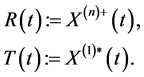
The evolution of the stock price process  is based on
 . Denote by
  the Best Bid and Ask(t) the Best Ask at time t. Then
  is the lowest price that a day trader seller is willing to accept for a stock at that time and Ask(t) is the highest price that a day trader buyer is willing to pay for that stock at any particular point in time. Let us define the processes
  and
and . Further set

where we use the convention that  and
and . Then
  and
and  can be modeled as
 (2)
(2)
and
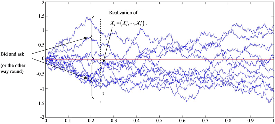
Figure 1. Realization of bid and ask.
 (3)
(3)
Given  and
and , the market makers will agree on a stock price within the Bid/Ask spread, that is
 (4)
(4)
where  is a stochastic process such that
  One could choose e.g.,
  for a function
  or
or  for a function
 .
.
For convenience, we will from now on assume that , that is
 (5)
(5)
3. Markovian Property of Processes R, T and S
For convenience, let us briefly discuss the Markovian property of the processes 
 and
and
 in some particular cases. The two cases considered here are the cases when the process
are Brownian motions or Ornstein-Uhlenbeck processes. Let us first have on the definition of semimartingales rank processes.
Definition 3.1 Let  be continuous semimartingales. For
 , the k-th rank process of
  is defined by
 (6)
(6)
where  and
and .
.
Note that, according to Definition 3.1, for ,
,
 (7)
(7)
so that at any given time, the values of the rank processes represent the values of the original processes arranged in descending order (i.e. the (reverse) order statistics).
Using Definition 3.1, we get
 (8)
(8)
3.1. The Brownian Motion Case
Here we assume that the processes  are independent Brownian motions.
Proposition 3.2 The process  possesses the Markov property with respect to the filtration
 .
.
Proof. Let  be a one-dimensional Brownian motion. We first prove that
  is a Markov process. Define the process

Then  is a two dimensional Feller process.
Let . One observes that
  is a continuous and open map. Thus is follows from [14] (Remark 1, p. 327) that
  is a Feller process, too.
The latter argument also applies to the n-dimensional case, that is  is a Feller process. Since

is a continuous and open map we conclude that  is a Feller process.
Proposition 3.3 The process  possesses Markov property with respect to the filtration
 .
.
Proof. See the proof of Proposition 3.2. 
Corollary 3.4 The process  possesses Markov property with respect to the filtration
 .
.
Proof. The process  defined by
  for all
  is a Markov process as sum of two Markov processes.
3.2. The Ornstein-Uhlenbeck Case
Here we assume that the process  is an n-dimensional Ornstein-Uhlenbeck, that is
 (9)
(9)
where  and
and  are parameters. It is clear that an Ornstein-Uhlenbeck process is a Feller process. So we obtain Proposition 3.5 The process
  and
and  defined by (8) and (5) possess Markov property.
Proof. The conclusion follows from the proof of Proposition 3.2. 
Remark 3.6 Using continuous and open transformations of Markov processes, the above results can be generalized to the case, when the bid and ask processes are Feller processes. See [14].
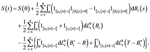
4. Further Properties of S(t)
In this Section, we want to use the semimartingale decomposition of our price process  to analyze completeness and arbitrage on market driven by such a process.
We need the following result. See [15] (Proposition 4.1.11). See also [16] for the continuous semimartingales case and [17] for general semimartingales.
Theorem 4.1 Let  be continuous semimartingales of the form (1). For
  let
let  be any predictable process with the property:
 (10)
(10)
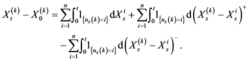
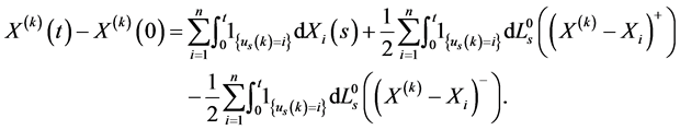
Then the k-th rank processes , are semimartingales and we have:
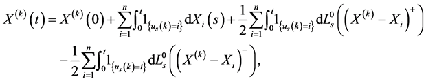 (11)
(11)
where  is the local time of the semimartingale
  at zero, defined by

where .
.
For completeness, we give the proof of the proposition.
Proof. We find that
 (12)
(12)
where we used the property . It follows,
We note the fact
 (13)
(13)
We now use the following formula:
 (14)
(14)
which is valid for non-negative semimartingales . See, e.g., [15,18]
Then, by applying (14) to , (12) becomes:
Then proof is completed.
4.1. The Brownian Motion Case
If  are
are  independent Brownian motions, the evolution of
  and
and  follows from Theorem 4.1.
Corollary 4.2 Let the processes  and
and  be given by Equation (8). Then
  and
and  and we have:
 (15)
(15)
and
 (16)
(16)
We can rewrite  and
and  as follows:
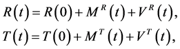
where  are continuous local martingales and
  are continuous processes of locally bounded variation given by:
 (17)
(17)
 (18)
(18)
 (19)
(19)
 (20)
(20)
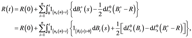
The following corollary gives the semimartingale decomposition satisfied by the process .
.
Corollary 4.3 Assume that the process  is given by (5). Then one can write
where  and
and , and we have:
 (21)
(21)
In order to price options with respect to , one should ensure that
  does not admit arbitrage possibilities and the natural question which arises at this point is the following: Can we find an equivalent probability measure
  such that,
  is a
is a  -sigma martingale? Since the process
  is continuous, we can reformulate the question as: Can we find an equivalent probability measure
  such that,
  is a
is a  local martingale1?
We first give the following useful remark; See [19] (Theorem 1).
Remark 4.4 Let  be a continuous semimartingale on a filtered probability space
 . Let
. Let . A necessary condition for the existence of an equivalent martingale measure is that
 .
.
Consequence 4.5 Since local time is singular, we observe that the total variation of the bounded variation part in 21 cannot be absolutely continuous with respect to the quadratic variation of the martingale. It follows that, the set of equivalent martingale measures is empty, and thus, such a market contains arbitrage opportunities.
4.2. (In)complete Market with Hidden Arbitrage
In this Section, we consider a model with , denoting a stochastic process modeling the price of a risky asset, and
  denotes the value of a risk free money market account. We assume a given filtered probability space
 , where
  satisfies the “usual hypothesis”. In such a market, a trading strategy
  is self-financing if
  is predictable,
  is optional, and
 (22)
(22)
for all . For simplicity, we let
  and
and  (thus the interest rate
 ), so that
 , and (22) becomes

Definition 4.6 (See [13])
• We call a random variable  a contingent claim. Further, a contingent claim
  is said to be
  -redundant if, for a probability measure
 , there exists a self-financing strategy
  such that
 (23)
(23)
where  is the value of the portfolio.
• A market  is
is  -complete if every
  is
is  -redundant.
Define the process  as follows
 (24)
(24)
Then the following theorem is immediate from [13] (Theorem 3.2).
Theorem 4.7 Suppose that there exists a unique probability measure  equivalent to
  such that
  is a
is a  -local martingale. Then, the market
  is
is  -complete.
Proof. Omitted. 
Proposition 4.8 Suppose that . Then, there exists no unique martingale measure
  such that
  is a
is a  -local martingale.
Proof. From (24), we observe that  is a
is a  -martingale. Let us construct another equivalent martingale measure
  For this purpose, assume without loss of generality that
  and
and  are given by

and

Now define the process  as
as

where

with
 (25)
(25)
One finds that  for all
 . Let us define the equivalent measure
  with respect to a density process
  given by

Here,  denotes the Doléans-Dade exponential of the martingale
  defined by

Then, it follows from the Girsanov-Meyer theorem (see [20]) that  has a
has a  -semimartingale decomposition with a bounded variation part given by
  We have that

Since , it follows that

Thus  is a
is a  -martingale. Since
  is also a martingale measure with
 , the result follows.
Remark 4.9 In the case  (a single Bid/Ask), the market becomes complete since the process
 , defined by Equation (25) in the proof is equal to
 . Therefore the unique martingale measure is
 .
.
We can then deduce the following theorem on our process .
.
Theorem 4.10 Suppose that  and
and  are given by (21) and (24), respectively. Then
• For  (a single Bid/Ask), the market
  is
is  -complete and admits the arbitrage opportunity (26).
• For  (more than a single Bid/Ask), the market
  is incomplete and arbitrage exists.
Proof. From Theorem 4.8, we know that the market is  -complete for
  and incomplete for
 . Let
. Let  such that
  is a
is a  -local martingale. For
 , let us construct an arbitrage strategy. Let
 (26)
(26)
where  denotes the
  by
by  support of the (random) measure
 ; that is, for fixed
  it is the smallest closed set in
  such that
  does not charge its complement. (Compare with the proof of Proposition 4.8.) Let

Assume without loss of generality that . Then, by Theorem 4.7, there exists a self financing strategy
  such that
  However, from (26), we also have
 Moreover, we have
 , by construction of the process
 .
.
Hence,  which is an arbitrage opportunity.
Remark 4.11 We do not make the assumption that we are working in an arbitrage free market, rather, we define the notion of redundancy (see [13] Definition 2.1), which in some sense is equivalent to the notion of replication with the difference that, replication is on a arbitrage free setting.
5. Pricing and Insider Trading with Respect to S(t)
In this Section, we discuss a framework introduced in [21], which enables us pricing of contingent claims with respect to the price process  of the previous sections. We even consider the case of insider trading, that is, the case of an investor, who has access to insider information. To this end, we need some notions.
We consider a market driven by the stock price process  on a filtered probability space
 . We assume that, the decisions of the trader are based on market information given by the filtration
  with
with  for all
  being a fixed terminal time. In this context an insider strategy is represented by an
  -adapted process
  and we interpret all anticipating integrals as the forward integral; See, for e.g., [22,23] for more details. In such a market, a natural tool to describe the self-financing portfolio is the forward integral of an integrand process
  with respect to an integrator
 denoted by
 ; See [23]. The following definitions and concepts are consistent with those given in [21].
Definition 5.1 A self-financing portfolio is a pair , where
  is the initial value of the portfolio and
  is a
is a  -adapted and
  -forward integrable process specifying the number of shares of held in the portfolio. The market value process
  of such a portfolio at time
 , is given by
 (27)
(27)
while  constitutes the number of shares of the less risky asset held.
5.1.  -Martingales
Now, we briefly review the definition of  -martingales which generalizes the concept of a martingale. We refer to [21] for more information about this notion. Throughout this Section,
  will be a real linear space of measurable processes indexed by
  with paths which are bounded on each compact interval of
 .
.
Definition 5.2 A process  is said to be a
  -martingale, if every
  in
in  is
is  -improperly forward integrable and
 (28)
(28)
Definition 5.3 A process  is said to be
  -semimartingale if it can be written as the sum of an
  -martingale
  and a bounded variation process
 , with
 .
.
• Remark 5.4
• Let  be a continuous
  -martingale with
  belonging to
 , then, the quadratic variation of
exists improperly. In fact, if  exists improperly, then one can show that
  exists improperly and
 .
.
• Let  a continuous square integrable martingale with respect to some filtration
 . Suppose that every process in
  is the restriction to
  of a process
  which is
  -adapted. Moreover, suppose that its paths are left continuous with right limits and
 . Then
  is an
is an  -martingale.
5.2. Completeness and Arbitrage:  -Martingale Measures
The subsequent definitions and notions are from [21].
Definition 5.5 Let  be a self-financing portfolio in
 , which is
  -improperly forward integrable and
  its wealth process. Then
  is an
is an  -arbitrage if
  exists almost surely,
  and
and 
Definition 5.6 If there is no  -arbitrage, the market is said to be
  -arbitrage free.
Definition 5.7 A probability measure  is called a
  -martingale measure if with respect to
  the process
  is an
is an  -martingale according to Definition 5.2.
We need need the following assumption. See [21].
Assumption 5.8 Suppose that for all  in
in  the following condition holds. Then
  is
is  -improperly forward integrable and
 (29)
(29)
The proof of the following proposition can be found in [21].
Proposition 5.9 Under Assumption 5.8, if there exists an  -martingale measure
 , the market is
  -arbitrage free.
Definition 5.10 A contingent claim is an  -measurable random variable. Let
  be the set of all contingent claims the investor is interested in.
• Definition 5.11
• A contingent claim  is called
  -attainable if there exists a self-financing trading portfolio
  with
with  in
in , which is
  -improperly forward integrable, and whose terminal portfolio value coincides with
 , i.e.,
Such a portfolio strategy  is called a replicating or hedging portfolio for
  and
and  is the replication price for
 .
.
• A  -arbitrage free market is called
  -complete if every contingent claim in
  is attainable.
Assumption 5.12 For every  -measurable random variable
 , and
, and  in
in  the process
 , belongs to
 .
.
Proposition 5.13 Suppose that the market is  -arbitrage free, and that Assumption 5.8 holds. Then the replication price of an attainable contingent claim is unique.
Proof. Let  be a given measure equivalent to
 . For such a
 , let
, let  be a set of all strategies (
 - adapted) such that (28) in Definition 5.2 is satisfied. Then, it follows from Proposition 5.9 that the market
  in Section 4.2 is
  -arbitrage free.
Next, we shall discuss attainability of claims in connection with a concrete set  of trading strategies.
5.3. Hedging with Respect to S(t)
In this Section, we want to determine hedging strategies for a certain class of European options with respect to the price process  of Section 4.2. Let us now assume that
  (a single Bid/Ask). Then, the price process
  is the sum of a Wiener process and a continuous process with zero quadratic variation; moreoverwe have that
 , where
  is given by (25). We can derive the following proposition which is similar to [21] (Proposition 5.29).
Proposition 5.14 Let  be a function in
  of polynomial growth. Suppose that there exist
 of class
  which is a solution of the following Cauchy problem
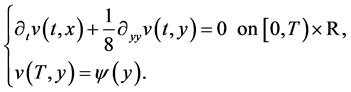 (30)
(30)
Set

Then  is a self-financing portfolio replicating the contingent claim
 .
.
In particular,  is
is  -complete, where
  is given by
and  by all claims as stated in this Proposition.
Proof. The proof is a direct consequence of Itô’s Lemma for forward integrals. See [21] (Proposition 5.29).
6. Conclusion
In this paper, assuming that the dynamics of the bid and ask prices are given by Itô processes, we derive the stochastic differential equation satisfied by the “best bid” and the “best ask” from which we get the dynamic of the middle (stock) price. The evolution of the latter is given by a semimartingale, whose final variation part, is not absolute continuous with respect to the Lebesgue measure. We then show that, such a market admits a hidden arbitrage opportunity and compute the arbitrage strategy. We also discuss the notion of (insider) hedging in this market.
REFERENCES
- J. Harrison and D. Kreps, “Martingales and Arbitrage in Multiperiod Securities Markets,” Journal of Economic Theory, Vol. 20, No. 3, 1979, pp. 381-408. http://dx.doi.org/10.1016/0022-0531(79)90043-7
- J. Harrison and S. Pliska, “Martingales and Stochastic Integrals in the Theory of Continuous Trading,” Stochastic Processes and Their Applications, Vol. 11, No. 3, 1979, pp. 215-260. http://dx.doi.org/10.1016/0304-4149(81)90026-0
- D. M. Kreps, “Arbitrage and Equilibrium in Economics with Infinitely Many Commmodities,” Journal of Mathematical Economics, Vol. 8, No. 1, 1981, pp. 15-35. http://dx.doi.org/10.1016/0304-4068(81)90010-0
- J. Bion-Nadal, “Bid-Ask Dynamic Pricing in Financial Markets with Transaction Costs and Liquidity Risk,” Journal of Mathematical Economics, Vol. 45, No. 11, 2009, pp. 738-750. http://dx.doi.org/10.1016/j.jmateco.2009.05.004
- E. Jouini and H. Kallal, “Martingales and Arbitrage in Security Market with Transaction Coast,” Journal of Economic Theory, Vol. 66, No. 1, 1995, pp. 178-197. http://dx.doi.org/10.1006/jeth.1995.1037
- A. Cherny, “General Arbitrage Pricing Model. II. Transaction Costs,” In C. Donati-Martin, M. Emery, A. Rouault and C. Stricker, Eds., Séminaire de Probabilités XL, Volume 1899 of Lecture Note in Mathematics, Springer, Berlin, Heidelberg, 2007, pp. 447-461.
- P. Carr, H. Geman and D. Madan, “Pricing and Hedging in Incomplete Markets,” Journal of Financial Economics, Vol. 62, No. 1, 2001, pp. 131-167. http://dx.doi.org/10.1016/S0304-405X(01)00075-7
- H. Föllmer and A. Schield, “Stochastic Finance: An Introduction in Discrete Time,” 2nd Edition, De Gruyter Studies in Mathematics, Berlin, New York, 2004.
- N. El Karoui and M. C. Quenez, “Dynamic Programming and the Pricing of Contingent Claims in Incomplete Markets,” SIAM Journal on Control and Optimization, Vol. 33, No. 1, 1995, pp. 29-66. http://dx.doi.org/10.1137/S0363012992232579
- N. El Karoui, S. Peng and M. C. Quenez, “Backward Stochastic Differential Equations in Finance,” Mathematical Finance, Vol. 7, No. 1, 1997, pp. 1-77. http://dx.doi.org/10.1111/1467-9965.00022
- S. Peng, “Non Linear Expectation, Nonlinear Evaluation and Risk Measure, Volume 1856 of Lecture Notes in Mathematics,” Springer, Berlin, Heidelberg, 2004, pp.165-253.
- S. Peng, “Modelling Derivatives Pricing Mechanisms with Their Generating Functions,” 2006. http://arxiv.org/pdf/math/0605599v1.pdf
- R. Jarrow and P. Protter, “Large Traders, Hidden Arbitrage, and Complete Markets,” Journal of Banking & Finance, Vol. 29, No. 11, 2005, pp. 2803-2820. http://dx.doi.org/10.1016/j.jbankfin.2005.02.005
- E. B. Dynkin, “Markov Processes, Volume 1,” Springer-Verlag, Berlin, Göttigen, Heidelberg, 1965.
- R. Fernholz, “Stochastic Portfolio Theory,” Springer-Verlag, Berlin, 2002. http://dx.doi.org/10.1007/978-1-4757-3699-1
- A. D. Banner and R. Ghomrasni, “Local Times of Ranked Continuous Semimartingales,” Stochastic Processes and their Applications, Vol. 118, No. 7, 2008, pp. 1244-1253. http://dx.doi.org/10.1016/j.spa.2007.08.001
- R.Ghomrasni and O. Menoukeu-Pamen, “Decomposition of Order Statistics of Semimartingales Using Local Times,” Stochastic Analysis and Applications, Vol. 28, No. 3, 2010, pp. 467-479. http://dx.doi.org/10.1080/07362991003708341
- R. J. Chitashvili and M. G. Mania, “Decomposition of the Maximum of Semimartingales and Generalized Itô’s Formula” In: V. V. Sazonov and T. L. Shervashidze, Eds., New Trends in Probability and Statistics, Volume 1, Proceedings of the Bakuriani Colloquium in Honour of Yu. V. Prohorov, USSR, Bakuriani, 24 February-4 March 1990, pp. 301-350.
- P. Protter and K. Shimbo, “No Arbitrage and General Semimartingales,” In: Markov Processes and Related Topics: A Festschrift for Thomas G. Kurtz, Volume 4, Institute of Mathematical Statistics, Beachwood, 2008, pp. 267-283.
- P. Protter, “Stochastic Integration and Differential Equations,” 2nd Edition, Springer-Verlag, Berlin, 2005. http://dx.doi.org/10.1007/978-3-662-10061-5
- R. Coviello and F. Russo, “Modeling Financial Assets without Semimartingale,” 2006. http://arxiv.org/pdf/math/0606642.pdf
- D. Nualart and E. Pardoux, “Stochastic Calculus with Anticipating Integrands,” Probability Theory and Related Fields, Vol. 78, 1988, pp. 535-581. http://dx.doi.org/10.1007/BF00353876
NOTES

1In fact since S is continuous and since all continuous sigma martingales are in fact local martingales, we only need to concern ourselves with local martingales