Journal of Mathematical Finance
Vol.3 No.2(2013), Article ID:31802,12 pages DOI:10.4236/jmf.2013.32025
Mixed Band Control of Mutual Proportional Reinsurance*
1Department of Mathematics, University of Missouri, Columbia, USA
2College of Business, City University of Hong Kong, Hong Kong, China
3Center for Transport, Trade and Financial Studies, City University of Hong Kong, Hong Kong, China
Email: liujjp@gmail.com, #laser.yuan@gmail.com
Copyright © 2013 Michael Taksar et al. This is an open access article distributed under the Creative Commons Attribution License, which permits unrestricted use, distribution, and reproduction in any medium, provided the original work is properly cited.
Received January 3, 2013; revised March 26, 2013; accepted April 9, 2013
Keywords: Insurance and Risk Management; Dynamic Programming and Control
ABSTRACT
In this paper, we investigate the optimization of mutual proportional reinsurance—a mutual reserve system that is intended for the collective reinsurance needs of homogeneous mutual members, such as P&I Clubs in marine mutual insurance and reserve banks in the US Federal Reserve, where a mutual member is both an insurer and an insured. Compared to general (non-mutual) insurance models, which involve one-sided impulse control (i.e., either downside or upside impulse) of the underlying insurance reserve process that is required to be positive, a mutual insurance differs in allowing two-sided impulse control (i.e., both downside and upside impulse), coupled with the classical proportional control of reinsurance. We prove that a special band-type impulse control 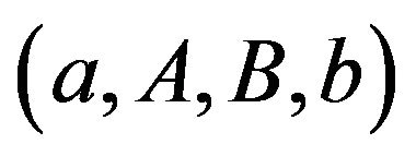 with
with  and
and , coupled with a proportional reinsurance policy (classical control), is optimal when the objective is to minimize the total maintenance cost. That is, when the reserve position reaches a lower boundary of
 , the reserve should immediately be raised to level A; when the reserve reaches an upper boundary of b, it should immediately be reduced to a level B. An interesting finding produced by the study reported in this paper is that there exists a situation such that if the upside fixed cost is relatively large in comparison to a finite threshold, then the optimal band control is reduced to a downside only (i.e., dividend payment only) control in the form of
  with
with . In this case, it is optimal for the mutual insurance firm to go bankrupt as soon as its reserve level reaches zero, rather than to jump restart by calling for additional contingent funds. This finding partially explains why many mutual insurance companies, that were once quite popular in the financial markets, are either disappeared or converted to non-mutual ones.
1. Introduction
This study is motivated by the long lasting while still strong-going success of marine mutual insurance (e.g., a P&I club of ship owners), the longest in the insurance business with a history of over 200 years; and by the still unanswered question why the once popular mutual insurance firms almost disappeared after 1990’s, either went bankrupt or converted to commercial (non-mutual) insurance business. A client of a mutual insurance is both insurer and insured, under a unique contingent regulation scheme of two-way impulse control (termed band control) which we give a brief description as follows. A mutual insurance firm is allowed: 1) to make calls for contingent injection from its clients once the reserve level is considered too low, as opposed to a commercial (non-mutual) insurance firm which would go bankrupt once its reserve becomes depleted; 2) or to make refunds (pay dividends) to its clients if the reserve is considered too high. We shall note that it is also permissible to adjust premium rate and liability policy in the continuous time horizon in conjunction of the band control as just mentioned, which in this case is referred to as a mixed band control of insurance reserves (i.e., a band type impulse control mixed with time-continuous classical control of a reserve process). Although in practice, mutual insurance engages mixed band control, most studies in the current literature are focused on the band control only, without classical control (e.g., with given constant premium rate, see [1,2] for reference). In this paper we consider mixed band control of mutual reinsurance which provides insurance to other mutual insurance firms, such as P&I clubs, of which each insures a number of ship-owners.
Reinsurance has been long investigated as an intrinsic part of commercial insurance, of which the mainstream modeling framework is profit maximization with the one-sided impulse control of an underlying reserve process. There are two types of one-sided impulse control: downside-only impulse control (such as a dividend payment) with a fixed cost  (e.g., Cadenillas et al. [3], Hojgaard and Taksar [4]) and upside-only impulse control (such as inventory ordering) with a fixed cost
  (e.g., Bensoussan et al. [2], Eisenberg and Schmidli [5], Sulem [6]). In this paper, we examine mutual proportional reinsurance—a mutual reserve system that is intended for the collective reinsurance needs of homogeneous mutual members, such as the P&I Clubs in marine mutual insurance (e.g., Yuan [7]) and the reserve banks in the US Federal Reserve (e.g., Dawande et al. [8]). A mutual insurance differs from a general (non-mutual) insurance in two key dimensions: 1) a mutual system is not for profit, and 2) a mutual reserve involves two-sided impulse control (i.e., both a dividend refund as a downside impulse to decrease the reserve with cost
  and a call for funds as an upside impulse to increase the reserve with cost
 ). It should be noted that the reserve process for a general insurance must always be positive (above zero), and the insurance firm is considered bankrupt as soon as its reserve falls to zero.
The mutual proportional reinsurance model developed in this paper is a generalization of the proportional reinsurance models (e.g., Cadenillas et al. [3], Hojgaard and Taksar [4], Eisenberg and Schmidli [5], Løkka and Zervos [9]) and is modified with the two differing characteristics noted above. More specifically, the proportional reinsurance rate can be adjusted in continuous time, and the underlying mutual reserve process is regulated by a two-sided impulse control in terms of a contingent dividend payment (i.e., a downside impulse control to decrease the mutual reserve level) and contingent call for contributions (i.e., an upside impulse control to increase the mutual reserve level). The corresponding mathematical problem for mutual proportional reinsurance becomes a two-sided impulse control system combined with a classical rate control in continuous time, a problem yet to be posed in insurance research. A problem that involves a mix of impulse control and classical control is termed a hybrid control problem in control theory, of which the difficulty has been well noted (e.g., Bensoussanand Menaldi [10], Branicky, Borkarand Mitter [11], Abate et al. [12]).
A pure two-sided impulse control problem (i.e., without a classical rate control) was investigated by Constantinides [13] in the form of cash management. Constantinides and Richard [1] showed an optimal two-sided impulse control policy to exist in the form of a band control, denoted with four parameters as  with
with . In other words, when the reserve position reaches a lower boundary a, then the reserve should immediately be raised to level A; when the reserve reaches upper boundary b, it should immediately be reduced to level B. For our mutual proportional reinsurance problem, we specify the corresponding Hamilton-Jacobi-Bellman (HJB) equation and the associated quasi-variational inequalities (QVI), from which we analytically solve the optimal value function. We then prove that a special band-type impulse control
  with
with , combined with a proportional reinsurance policy (classical control), is optimal when the objective is to minimize the total maintenance cost. An interesting finding reported here is that there exists a situation such that if the upside fixed cost
  is relatively large in comparison to a finite threshold
 , then the optimal band control is reduced to a downside only (i.e., a dividend payment only) control in the form of
  with
with . In this case, it is optimal for the mutual insurance to go bankrupt as soon as its reserve level falls to zero, rather than to restart by calling for additional contingent funds. This finding partially explains why many mutual insurance companies, that were once quite popular in the financial markets, are either disappeared or converted to non-mutual ones.
The remainder of the paper is organized as follows. In Section 2, we formulate the mathematical model and specify the HJB equation and the QVI of the corresponding stochastic control problem. We solve the QVI for the optimal value function in Section 3. In Section 3.2, we characterize and analyze the threshold . In Section 4, we prove the verification theorem and verify the optimal control. Finally, we make concluding remarks in Section 5.
2. The Model
2.1. Feasible Control
The classical Cramer-Lundberg model of an insurance reserve (surplus) is described via a compound Poisson process:
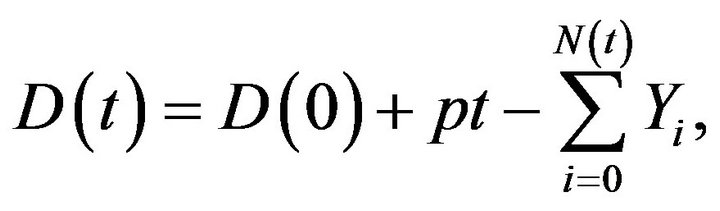
where  is the amount of the surplus available at time
 , quantity
  represents the premium rate,
  is the Poisson process of incoming claims and
  is the size of the ith claim. This surplus process can be approximated by a diffusion process with drift
  and diffusion coefficient
 , where
  is the intensity of the Poisson process
 . We assume that the insurer always sets
  (i.e.
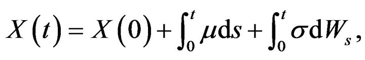
(i.e. ). Thus, with no control, the reserve process
  is described by
 (2.1)
(2.1)
where  is a standard Brownian motion.
We start with a probability space , that is endowed with information filtration
  and a standard Brownian motion
  on
on  adapted to
 . Two types of controls are used in this model. The first is related to the ability to directly control its reserve by raising cash from or making refunds to members at any particular time. The second is related to the mutual insurance firm’s ability to delegate all or part of its risk to a reinsurance company, simultaneously reducing the incoming premium (all or part of which is in this case channeled to the reinsurance company). In this model, we consider a proportional reinsurance scheme. This type of scheme corresponds to the original insurer paying u fraction of the original claim. The premium rate coming to the original insurer is simultaneously reduced by the same fraction. The reinsurance rate can be chosen dynamically depending on the situation.
Mathematically, control U takes a triple form:
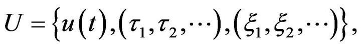 (2.2)
(2.2)
where  is a predictable process with respect to
 , the random variables
  constitute an increasing sequence of stopping times with respect to
 , and
, and  is a sequence of
  -measurable random variables,
 .
.
The meaning of these controls is as follows. The quantity  represents the fraction (reinsurance share) of the premium and risk (loss) incurred by the mutual insurance at time
 . Suppose that
  is chosen at time
 . Then, in the diffusion approximation (2.1), drift
  and diffusion coefficient
  are reduced by factor
  (see Cadenillas et al. [14], Hojgaard and Taksar [4]).
The fact that the process  is adapted to information filtration means that any decision has to be made on the basis of past rather than the future information. The stopping times
  represent the times when the ith intervention to change the reserve level is made. If
 , then the decision is to raise cash by calling the members/ clients. If
 , then the decision is to make a refund. The fact that
  is a stopping time and
  is
is  measurable also indicates that the decisions concerning when to make a contingent call and how much cash to raise are made on the basis of only past information. The same applies to the refund decisions.
Once control U is chosen, the dynamics of the reserve process becomes:
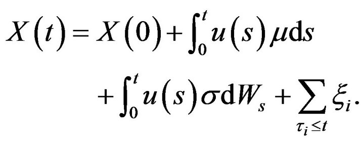 (2.3)
(2.3)
Define the ruin time as
 (2.4)
(2.4)
Control  is called admissible for initial position
  if, for
  for any
 ,
,
 (2.5)
(2.5)
and if
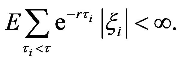 (2.6)
(2.6)
We denote the set of all admissible controls by .
.
The meaning of admissibility is as follows. At any time the decision to make a refund is made, the refund amount cannot exceed the available reserve. As can be seen in the following, if this condition is not satisfied, then one can always achieve a cost equal to , simply by making an infinitely large refund. The second condition of admissibility is a rather natural technical condition of integrability.
2.2. Cost Structure and Value Function
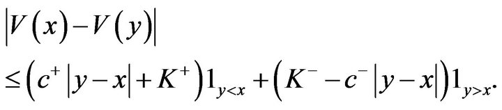
The objective in this model is to minimize the operational cost and the lost opportunity to invest the money in the market. Cost function  is defined as
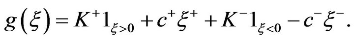 (2.7)
(2.7)
Here,  and
and  denote the positive and negative components of
 , that is,
  and
and  . The costs associated with refunds are of a different nature. A contingent call always increases the total cost, whereas a refund decreases it. However fixed set-up costs
  and
and  are incurred regardless of of the size of a contingent call or a refund. In addition, when the call is made and the cash is raised, there is a proportional cost associated with the amount raised. The constant
  represents the amount of cash that needs to be raised in order for one dollar to be added to the reserve. If the reserve is used for a refund, then a part of it may be charged as tax. The constant
  represents the amount actually received by the shareholders for each dollar taken from the reserve.
Given a discount rate r, the cost functional associated with the control U is defined as
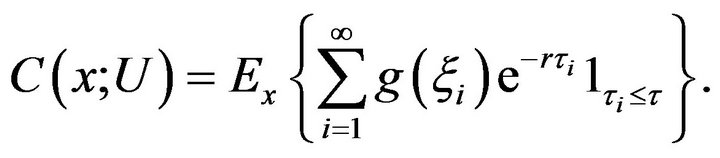 (2.8)
(2.8)
The objective is to find the value function,
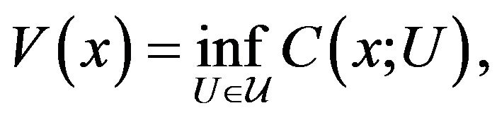 (2.9)
(2.9)
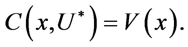
and optimal control , such that

2.3. Variational Inequalities for the Optimal Value Function
For each , define the infinitesimal generator
 . For any twice continuously differentiable function
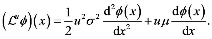 (2.10)
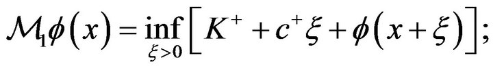
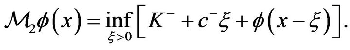
Let  be the inf-convolution operator, defined as
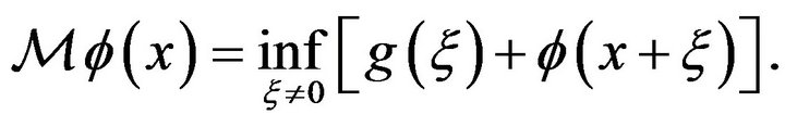 (2.11)
Definition 2.1. The QVI of the control problem are
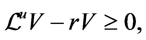 (2.12)
and
 (2.13)
together with the tightness condition
 (2.14)
3. Solution of the QVI
Before you begin to format your paper, first write and save the content as a separate text file. Keep your text and graphic files separate until after the text has been formatted and styled. Do not use hard tabs, and limit use of hard returns to only one return at the end of a paragraph. Do not add any kind of pagination anywhere in the paper. Do not number text heads—the template will do that for you.
Finally, complete content and organizational editing before formatting. Please take note of the following items when proofreading spelling and grammar:
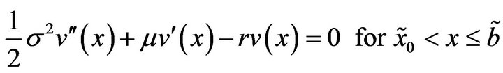
3.1. The HJB Equation in the Continuation Region
In this model, the application of the control that is related to calls and refunds results in a jump in the reserve process. This type of model is considered in the framework of the so-called impulse control. Because we also have a control whose application changes the drift and the diffusion coefficient of the controlled process, the resulting mathematical problem becomes a mixed regular-impulse control problem (e.g., Cadenillas et al. [14]). In the case of a pure impulse control, the optimal policy is of the  type, where the four parameters used to construct the optimal control must be computed as a part of a solution to the problem (see Cadenillas and Zapatero [15], Constantinides and Richard [10], Harrison and Taylor [16], and Paulsen [17]). Parameters
  and
and  represent the levels at which the intervention (application of impulses) must be made, whereas
  and
and  stand for the positions that the controlled process must be in after the intervention is made. This is a so-called band-type policy, with
  and
and  understood as the two bands that determine the nature of the optimal control. The interval
  is called the continuation region. When the process falls inside the continuation region, no interventions/impulses are applied. When an intervention is initiated, the time when the process reaches one of the boundaries of the continuation region corresponds to one of
 .
.
We conjecture that, in our case, the optimal intervention (impulse control) component of the problem is also of the band type. Moreover, as the following analysis implicitly shows, we can narrow our search for the optimal policy to a special band-type control , where the level
  associated with the contingent calls is set to zero. Therefore, only three of the four band-type policy parameters remain unknown. After finding these parameters (and determining the optimal drift/diffusion control in the continuation region), we will see that the cost function associated with this policy satisfies the QVI.
The derivation of the value function is similar to [3] and [14].Suppose that  satisfies all of the QVI conditions: (2.12), (2.13) and (2.14). First note that the function
  is a decreasing function of
 , and thus
 . To satisfy (2.14), for any
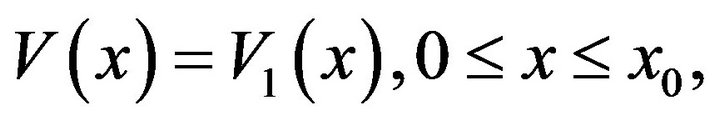
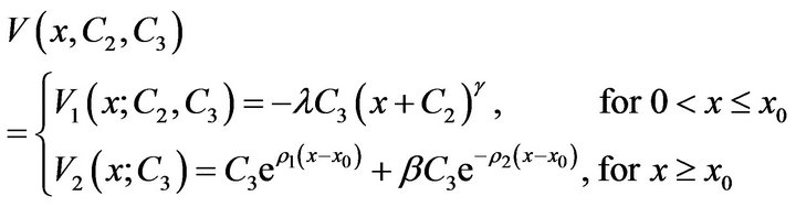
 , at least one of the two functions on the left side of the equation should be equal to zero. We conjecture that the value function has the following structure.
 (3.15)
for . Also
 (3.16)
for .
.
Assume that  minimizes the function
  in foregoing equation. If
  then
then
 (3.17)
provided that the right-hand side of (3.17) belongs to . (Note that if
 , then (3.16) cannot be satisfied and we exclude
  from consideration).
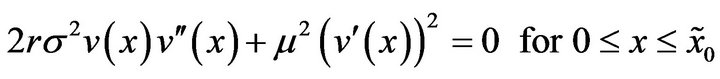
Substituting (3.17) into (3.16), we get
 (3.18)
The general solution for (3.18) is
 (3.19)
where  and
and  are free constants to be determined later, and
 (3.20)
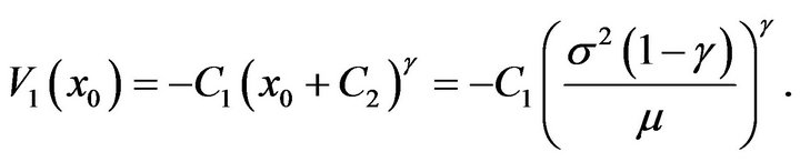
It is easy to see that . From (3.17), we obtain the expression for
  (provided that
  which will be verified later):
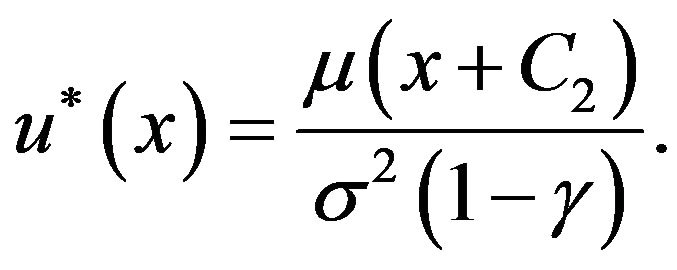 (3.21)
Note that the solution of (3.18) coincides with the solution of (3.16) only in the region where
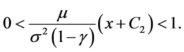
From this expression, we conjecture that there is a switching point  such that
  when
when . As
. As , by virtue of the equation (3.21), we obtain the following expression for
 :
:
 (3.22)
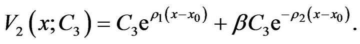
For ,
, ; and the corresponding differential equation becomes
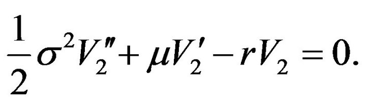 (3.23)
The general solution for (3.23) is
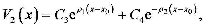 (3.24)
where
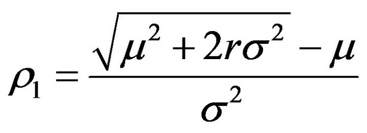 (3.25)
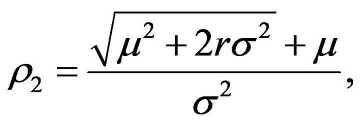 (3.26)
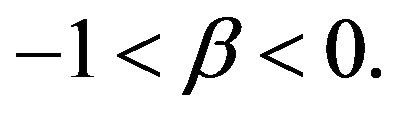
with . Standard arguments show that
 (3.27)
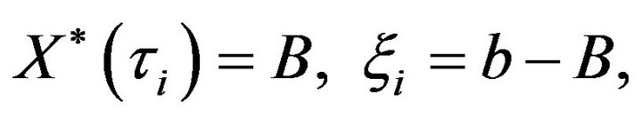
For  (see e.g., Cadenillas et al. [14]). The boundary conditions for the equation are rather tricky. If 0 and
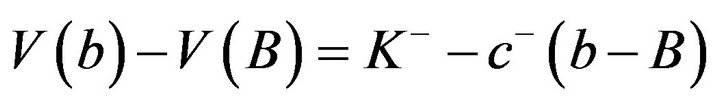
  are the points at which the impulse control (intervention) is initiated then the boundary conditions at these points become
 (3.28)
 (3.29)
 (3.30)
 (3.31)
However, if bankruptcy is allowed and no intervention is initiated when the process reaches 0, then the boundary condition at 0 becomes straightforward:  (see Cadenillas and Zapatero [3] and Cadenillas, et al. [14]). In our case, whether 0 is the point that corresponds to the intervention in the form of a contingent call or whether it corresponds to bankruptcy is not given a priori; rather it is part of the solution to the problem.
We seek the solution by finding a function  such that
 (3.32)
 (3.33)
 (3.34)
To find the free constants in the expressions for  an
an  and to paste different pieces of the solution together we apply the principle of smooth fit by making the value and the first derivatives to be continuous at the switching points
  and b,
 (3.35)
 (3.36)
 (3.37)
where  is defined by (3.22).
(It should be noted that the function , which is constructed from (3.32)-(3.34) subject to conditions (3.28)- (3.31) and (3.35)-(3.37), corresponds to the case in which the optimal policy leads to
 ). We begin by constructing such a function. The main technique is not to consider the function
  itself, but rather first to construct
 .
.
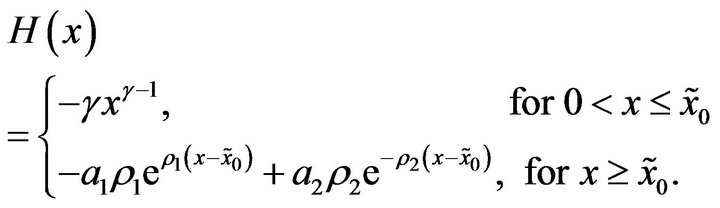
The form of  is shown in Figure 1.
From  and (3.17), we have
 . By the continuity on
  and
and  at
at , and by (3.23), we have
 . From this relation and (3.24), we have
Let . Then,
  , and we can write
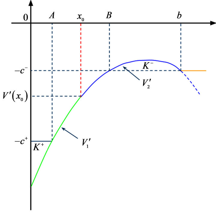
Figure 1. Optimal policy parameters.
We can easily get the inequalities:
 (3.38)
From (3.22), we get
From , and from the continuity of
  at
at , we obtain the expression for
 :
:
Let . (Obviously,
  since
since .) Now, we can write
  in terms of
  and
and :
:
What remains is to determine  and
and . Once these constants are found, we have
  and
and , and thus
 . Let
. Let
where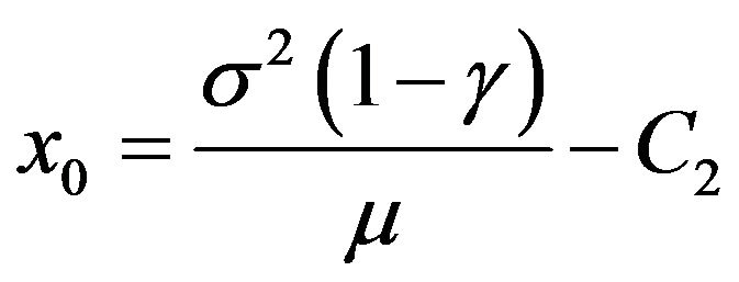 .
.
Note that if  and
and , then it is easy to show that for
 ,
,  ,
,
 and
and ,
,
 . Therefore,
  is decreasing on
  and
and  is concave on
 . In the remainder of this section, we find
  and
and  and complete the construction of the function
 . We do this in an implicit manner by adopting an auxiliary problem in which no contingent calls are allowed and by using the optimal value function of that problem to construct the function
 .
.
Let’s consider a slightly different problem in which only those controls  for which
  on the right-hand side of (2.2) are negative allowed. This problem is similar to that considered in Cadenillas et al. [14]. Let
  be the optimal value function for this problem. As was shown in [14], the function
  satisfies the same HJB equation, except for boundary conditions (3.28) and (3.29). These conditions are replaced by
 .
.
The same arguments as those above show that we can make the conjecture that the function  should be sought as a solution to (3.39)-(3.44) below.
 (3.39)
 (3.40)
 (3.41)
 (3.42)
 (3.43)
 (3.44)
where .
.
A Solution to the Auxiliary Problem
First note that a general solution to (3.39), (3.41) is , where
  is the same as in (3.20) and
  is a free constant, and a general solution to (3.40) is
 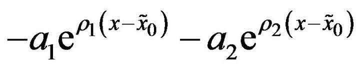 , where
  and
and  are the same as in (3.25), (3.26).
To solve our auxiliary problem we apply the same technique as that used in Cadenillas et al. [14]. We begin with , which is defined as follows.
 (3.45)
this expression, constants  and
and  are chosen in such a way that
  and
and
 . That is, the functions
  and
and  are continuous at
 . (Note that
  is a derivative of
  on
on  and
and  is a derivative of
  on
on .) We next examine the family of functions
 , where
 . We seek
  such that
  becomes the derivative of the optimal value function
 .
.
To this end, we start by finding points  and
and  such that
  and
and
 . Note that
  is a concave function, which is easily checked by differentiation. Let
 , the point at which the maximum of
  is achieved (it is easy to see that
 , whereas
 , which shows that
 exists; in view of the fact that
 , it is unique). It is obvious by virtue of the concavity of
  that, for any
 ,
,  and
and  exist.
We now consider . Informally,
  is the area under the graph of
  and above the horizontal line
 . It is obvious that
  is a continuous function of
 . For
. For , we have
 ; Let
; Let
Then,
 (3.46)
is the optimal value function of the auxiliary problem (see Figure 2). The proof here is identical to that of a similar statement in Cadenillas et al. [14] and thus we omit it.
3.2. The Optimal Value Function for the Original Problem
We employ the function  obtained in the previous subsection to construct the derivative of the optimal val-
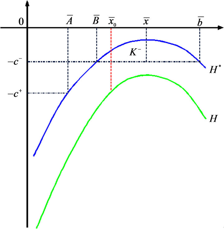
Figure 2. Solution to the auxiliary problem.
uefunction . The main idea is to consider
  and try to find
  such that
 . The optimal value function
  will then be sought in the form of
 . To this end, we need the following proposition.
Proposition 3.1. Suppose that  satisfies (3.39) (satisfies (3.40)); then, for any S, the function
  satisfies the same equation on the interval shifted by S to the left.
The proof of this proposition is straightforward.
From (3.45), we can see that  has a singularity at 0 with
 . The concavity of
  on
on
 implies that
  is increasing on
  and decreasing on
  (recall that
  is constant on
 ). Therefore, there exists unique
  such that
 . Define
 (3.47)
Note that  decreases to
  at 0 at the order of
  (see (3.45)); therefore,
  is integrable at 0 and, as a result,
 .
.
The qualitative nature of the solution to the original problem depends on the relationship between  and
and ; hence, we divide our analysis into two cases.
3.2.1. The Case of 
Consider the following integral
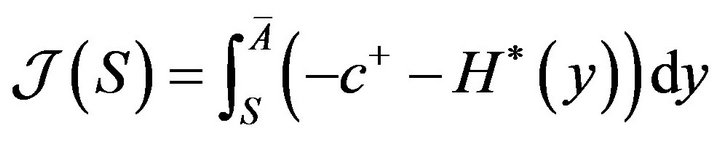
Geometrically this integral represents the area of a curvilinear triangle bounded by the lines ,
,  and the graph of the function
 . Obviously,
  is a continuous function of
 . Because
 and
and , there exists an
  (see
(see
Figure 3) such that
 (3.48)
In what follows, we show that  is the derivative of the solution
  to the QVI, inequalities (2.12)-(2.14).
Let
 (3.49)
Also let
 (3.50)
 (3.51)
 (3.52)
 (3.53)
 (3.54)
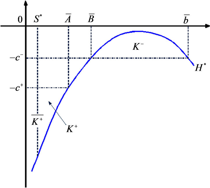
Figure 3. Determining the parameters for the value function  by utilizing the solution of the auxiliary problem
  when
when .
.
By virtue of Proposition 3.1, the function  satisfies (3.18) on
 , as well as (3.23) on
 . In addition, from (3.48), we can see that
 (3.55)
From the construction of the function , we can also see that
 (3.56)
We also have 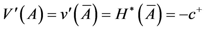 and similarly
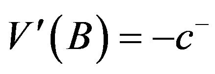 , so
, so  satisfies all the conditions (3.28)-(3.31).
Theorem 3.1. The function  given by (3.56) is a solution to the QVI (2.12)-(2.14).
The proof of this theorem is divided into several propositions.
Proposition 3.2. The function  satisfies (3.16) on
 .
.
Proof. 1) From the construction of the function v, we have  on
on . Consequently,
 (3.57)
on . As
. As  satisfies (3.18), it also satisfies (3.16) because these two equations are equivalent whenever (3.16) holds.
2) To prove that (3.16) holds for , it is sufficient to show that for each
 ,
,
 (3.58)
because, in view of Proposition 3.1, the function  satisfies (3.23) (that is,
 ). By subtracting (3.58) from the left hand side of (3.23), we can see that (3.58) is equivalent to
 (3.59)
for . In view of the continuity of the first and second derivatives, and in view of the fact that (3.16) holds on
 , we know that (3.59) is true for
 . As both
  and
and  on the left-hand side of (3.59) are decreasing, therefore is nonpositive for all
 .
.
Note that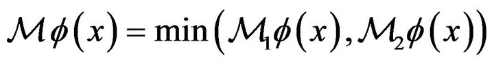 , where
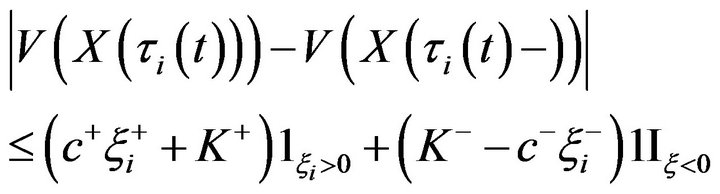
Proposition 3.3. For each , we have
 (3.60)
If , or if
 , then
 (3.61)
Proof. 1) We first prove, that . Supposethat
 . The function
  is continuously differentiable. By construction,
  is increasing on
  and decreasing on
  with
with  for
for . Therefore, the point
  is the only point
  such that
 . Because
 , we can see that
 . Therefore, for
 ,
,
Also,

if
However,

This proves that  for all
  and also shows that
 (3.62)
Because  for
for , we know that for any
  the function
  is an increasing function of
 . Therefore, the minimum in the expression for
  is attained for
 ; as a result,
 .
.
2) Consider  for
for . Because
  for
for  and
and  for
for , we can see that
  has a unique minimum at
 . Therefore,
 . Thus,
  if
if
The foregoing inequality always holds true because, by construction,
For , we note, that
 , and hence
 (3.63)
To complete the proof of Theorem 3.1, we need only show the following.
Proposition 3.4. If , then (2.12) holds.
Proof. It is sufficient to show that for any  and any
 ,
,
 (3.64)
From Proposition 3.2 we know that (3.64) is true for . As
. As , we obtain
 .
.
For any , we have

because V is a decreasing function. 
This completes the proof of Theorem 3.1.
3.2.2. The Case of 
When  we cannot find any S* such that (3.48) is satisfied. In this case, we set
  (that is, we have
 , which corresponds to
 ).
).
Theorem 3.2. If , then
  is a solution to the QVI (2.12)-(2.14).
To prove this theorem, it is sufficient to prove Propositions 3.2-3.4. The proofs of Propositions 3.2 and 3.4 are identical to the case of , whereas that of Proposition 3.3 requires a slight modification.
Proposition 3.5. For each ,
,
 (3.65)
If , then
 (3.66)
Proof. The proof that  for all
  and that
  for
for  is the same as that in Proposition 3.3.
If , then
  is equivalent to
The foregoing inequality is always true because
by assumption.
If , then
  still holds, due to the same argument as that in Proposition 3.3.
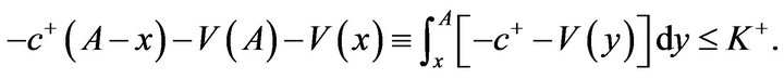
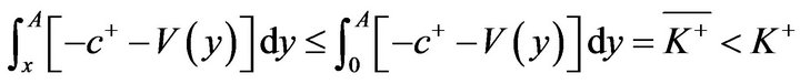
Remark 3.1. In the case of  we have
  only for
 , whereas
 in contrast to the case when
 . Also, when
 , we have
 , whereas
  if
if . Equivalently, in the case that the fixed cost to call for additional funds is relatively large (i.e.,
 ) , the optimal band control is reduced to
  with
with . That is, as soon as the reserve reaches zero, it becomes optimal for the mutual insurance firm to go bankrupt, rather than to be restarted by calling for additional funds.
4. Verification Theorem and the Optimal Control
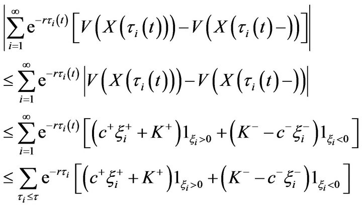
Theorem 4.1. If V is a solution to QVI (2.12)-(2.14), then for any control ,
,
 (4.67)
Proof. We prove this inequality when . In this case,
 . Let
. Let  be any admissible control defined by (2.2) and process
  be the corresponding surplus process (2.3), with
 . Let
. Let  be its ruin time given by (2.4). Let
  and
and . Then,
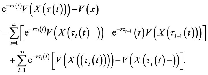 (4.68)
By convention, . In view of (2.13), we have
Therefore,
and
 (4.69)
In view of (2.6), this implies that for any  the second sum in (4.68) is bounded by the same integrable random variable independent of
 .
.
On , process
  is continuous, and we can apply Ito’s formula to get
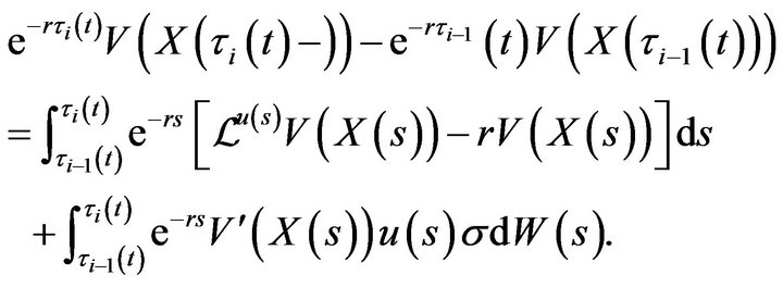 (4.70)
From this equation, using (2.6) and standard but rather tedious arguments, we can deduce that the first sum in (4.69) for all  is also bounded by the same integrable random variable. Similar arguments show that
 (4.71)
and
 (4.72)
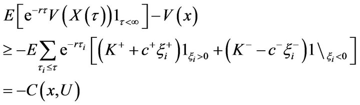
(see Cadenillas et al. [7]). Note that the second integral on the right-hand side of (4.70) is a martingale whose expectation vanishes. However, in view of (2.12), the integrand in the first integral of (4.70) is nonnegative. Therefore,
 (4.73)
and, taking into account the dominated convergence theorem, we can see that the expectation of the first sum on the right-hand side of (4.68) is nonnegative.
From (2.13), we can see that
Substituting this inequality into (4.2) and taking expectations of both sides, we obtain
 (4.74)
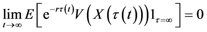
Letting , and employing (4.72) and the monotone convergence theorem on, we get
 (4.75)
As , on
, on , the inequality (4.75) implies (4.67).
Remark 4.1. For the expectation of the stochastic integral on the right hand side of (4.70) to vanish, it is sufficient for its integrand to be bounded. In particular, it is sufficient for  to be bounded. This is the case when
 . When
 , the function
  has a singularity at 0. We can, however, apply the same technique, first replacing
  by
by  and then passing to a limit as
 . This will yield inequality (4.74), which is all we need for the proof of Theorem 4.1 Let
 , that is
 (4.76)
From (3.46), (3.45), (3.49), and (3.53), we can see that
Consider the process defined as
 (4.77)
 , with
 ,
,  , and
, and  and
and  are defined below sequentially.
If  (that is, no
  exists, such that (3.48) holds), then
 (4.78)
where
 (4.79)
If  (that is, there exists an
 , such that (3.48) holds), then
 (4.80)
where
 (4.81)
Remark 4.2. Informally, if , then process
  is a continuous diffusion process with a drift and diffusion coefficient of,
  and
and  , respectively, until the times of intervenetion. The times of intervention in this case are the times at which this diffusion process hits the level
 , which are associated with the refunds of the constant amount of
 . The time when 0 is hit is the ruin time.
When , the process
  is a continuous diffusion process with the same drift and diffusion coefficients as above, between the times of intervention. The intervention times are the times at which this process reaches either 0 or
 . At point 0, the control is set to displace the process to point
 , which corresponds to raising cash (making a call to shareholders) in the amount of
 . Reaching the level
  results in the displacement of the process to the point
  which, corresponds to making a refund in the amount of
 .
.
Theorem 4.2. (The verification theorem) Let  be the control described by (4.76) and (4.79)-(4.80). Then,
Proof. In view of (4.67), it is sufficient to show that
 (4.82)
Equality (4.76) shows that
 (4.83)
From Propositions 3.3 and 3.5, we know that
 and if
  then
then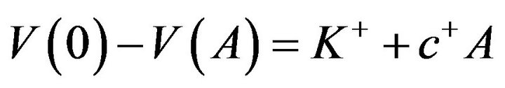 . Thus, we can repeat the arguments in the proof of Theorem 3.2 and see that, for
 , all of the inequalities are tight. As a result, we obtain
 (4.84)
Because we know that, when , we have
  and, when
 , the function V satisfies
 , the first term on the left-hand side of (4.84) vanishes, and we get (4.82).
5. Conclusions
The optimal policy in this model has several interesting nontrivial features. The fact that calls should be made only when there is no possibility of waiting any longer (that is when the reserve reaches zero) is supported by intuition. However, the qualitative structure of the optimal policy and its dependence on the model parameters are not as obvious.
It turns out that it is always optimal to pay dividends, no matter what the costs associated with such payments are. However, raising cash may not be optimal when the initial set-up cost is too high. Quantity , which determines the threshold for set-up cost
 , such that if the cost is higher than this threshold then it is optimal to allow ruin, is in itself determined via an auxiliary problem with a one-sided impulse control. Although there is no closed-form expression for the quantity
 , it can be determined in an algorithmic manner prior to solving the optimal control problem for the mutual insurance company.
There is one rather curious feature of the optimal solution when . As our analysis shows, in this case,
  and
and , the same as is the case when
 . However, from the construction of the optimal policy, we can see that the two band-type policy is optimal in this case as well. In this borderline case, we thus have two optimal policies, one for which
  with the lower band equal to
  and one for which reaching 0 corresponds to ruin and for which
 . This is a rather unique feature of this particular problem that has not been observed previously.
A natural question arises: what if ruin is explicitly disallowed, and we must find an optimal policy from among those for which . As can be seen from our analysiswe find a solution to this problem for the case of
 . However, when this inequality does not hold, then of the stochastic control technique and the HJB equation used in this paper do not work. Another approach should be developed, as can be seen indirectly in the work of Eisenberg [18] and Eisenberg and Schmidli [5], where a similar (although not identical) problem is considered for the case of a surplus process modeled via the classical Cramer-Lundberg model. This constitutes an interesting and challenging problem for future study, the nature of whose solution is not obvious at this time.
REFERENCES
- G. M. Constantinides, and S. F. Richard, “Existence of Optimal Simple Policies for Discounted-cost Inventory and Cash Management in Continuous Time,” Operations Research, Vol. 26, No. 4, 1978, pp. 620-636. doi:10.1287/opre.26.4.620
- A. Bensoussan, R. H. Liu and S. P. Sethi, “Optimality of an (s, S) Policy with Compound Poisson and Diffusion Demands: AQuasi-variationalInequalities Approach,” SIAM Journal on Control and Optimization. Vol. 44, No. 5, 2006, pp. 1650-1676. doi:10.1137/S0363012904443737
- A. Cadenillas and F. Zapatero, “Classical and Impulse Stochastic Control of the Exchange Rate Using Interest Rate and Reserves,” Mathematical Finance, Vol. 10, No. 2, 2000, pp. 141-156. doi:10.1111/1467-9965.00086
- B. M. Hojgaard and M. Taksar, “Optimal Dynamic Portfolio Selection for a Corporation with Controllable Risk and Dividend Distribution Policy,” Quantitative Finance, Vol. 4, No. 3, 2004, pp. 256-265. doi:10.1088/1469-7688/4/3/007
- J. Eisenberg and H. Schmidli,“Minimizing Expected Discounted Capital Injections by Reinsurance in a Classical Risk Model,” Scandinavian Actuarial Journal, No. 3, 2011,pp. 155-176. doi:10.1080/03461231003690747
- A. Sulem, “A Solvable One-dimensional Model of A Diffusion Inventory System,” Mathematics of Operations Research, Vol. 11, No. 1, 1986, pp. 125-133. doi:10.1287/moor.11.1.125
- J. Yuan, J, “Computational Optimization of Mutual Insurance Systems: A Quasi-variational Inequality Approach,” Ph.D. Thesis, The Hong Kong Polytechnic University, 2008.
- M. Dawande, M. Mehrotra, V. Mookerjee and C. Srikandarajah, “An Analysis of Coordination Mechanism for the U.S. Cash Supply Chain,” Management Science, Vol. 56, No. 3, 2010, pp. 553-570. doi:10.1287/mnsc.1090.1106
- A. Løkka and A. M. Zervos, “Optimal Dividend and Issuance of Equity Policies in the Presence of Proportional Costs,” Insurance: Mathematics and Economics, Vol. 42, No. 3, 2008, pp. 954-961. doi:10.1016/j.insmatheco.2007.10.013
- A. Bensoussan and J. L. Menaldi, “Stochastic HybridControl,” Journal of Mathematical Analysis and Applications, Vol. 249, No. 1, 2000, pp. 261-288. doi:10.1006/jmaa.2000.7102
- M. S. Branicky, V. S. Borkar and S. K. Mitter, “A Unified Framework for Hybrid Control: Model and Optimal Control Theory,” IEEE Transactions on Automatic Control, Vol. 43, No. 1, 1998, pp. 31-45. doi:10.1109/9.654885
- A. Abate, A. D. Ames and S. Sastry, “Stochastic Approximations for Hybrid Systems,” Proceedings of the 24th American Control Conference, Portland, 2005, pp. 1557-1562.
- G. M. Constantinides, “Stochastic Cash Management with Fixed and Proportional Transaction Costs,” Management Science, Vol. 22, No. 12, 1976, pp. 1320-1331. doi:10.1287/mnsc.22.12.1320
- A. Cadenillas, T. Choulli, M. Taksar and L. Zhang, “Classical and Impulse Stochastic Control for the Optimization of the Dividend and Risk Policies of an Insurance Firm,” Mathematical Finance, Vol. 16, No. 1, 2006, pp. 181-202. doi:10.1111/j.1467-9965.2006.00267.x
- A. Cadenillas and F. Zapatero, “Optimal Central Bank Intervention in the Foreign Exchange Market,” Journal of Economic Theory, Vol. 87, No. 1, 1999, pp. 218-242. doi:10.1006/jeth.1999.2523
- J. M. Harrison, T. M. Sellke and A. J. Taylor, “Impulse control of Brownian Motion,” Mathematics of Operations Research, Vol. 8, No. 3,1983, pp. 454-466. doi:10.1287/moor.8.3.454
- J. Paulsen, “Optimal Dividend Payments and Reinvestments of Diffusion Processes with Both Fixed and Proportional Costs,” SIAM Journal on Control and Optimization, Vol. 47, No. 5, 2008, pp. 2201-2226. doi:10.1137/070691632
- J. Eisenberg, “Optimal Control of Capital Injections by Reinsurance and Investments,” Blätter der DGVFM, Vol. 31, No. 2, 2010, pp. 329-345. doi:10.1007/s11857-010-0124-0.
NOTES
*This work was initiated by and is completed in memory of the late Professor Taksar.
This work is support in part by Hong Kong GRF522507E.
#Corresponding author.