Journal of Mathematical Finance
Vol.3 No.1A(2013), Article ID:29330,16 pages DOI:10.4236/jmf.2013.31A016
The Effects of Systemic Risk on the Allocation between Value and Growth Portfolios
Departamento de Economía y Empresa, Universidad CEU Cardenal Herrera, Valencia, Spain
Email: gonzalo.rubio@uch.ceu.es
Received November 1, 2012; revised December 14, 2012; accepted December 27, 2012
Keywords: Systemic Risk; Value; Growth; Asset Allocation; Risk Aversion
ABSTRACT
Given the striking effects of the recent financial turmoil, and the importance of value and growth portfolios for both local and international portfolio allocation, we investigate the effects of systemic jumps on the optimal portfolio investment strategies across value and growth equity portfolios. We find that the cost of ignoring systemic jumps is not substantial, unless the portfolio is highly levered and the average size amplitude of the jump is large enough. From the optimal asset allocation point of view, it seems more important the effects of few but relatively large jumps than highly frequent but small jumps. Indeed, the period in which the value premium is higher coincides with a period of few, but large and positive average size jumps for value stocks, and negative and very large average size jumps for growth stocks.
1. Introduction
The value premium is one of the most relevant anomalies discussed in the asset pricing literature. Value stocks, which are characterized by high book-to-market ratios, earn higher average returns than growth stocks. In principle, growth options strongly depend upon future economic conditions which suggest that growth stocks should have higher betas than value stocks. Using monthly data from January 1963 to December 2010, the market beta of the Fama-French growth portfolio is 1.067 while the market beta of the value portfolio is 1.068. Although contrary to the theoretical prediction these betas are basically the same, it turns out that the annualized average return of the growth portfolio is 9.6% while the annualized average return of the value portfolio is 16.5%. This represents a value premium of 6.9% which is even higher that the well known market equity premium magnitude of 5.5% for the same sample period.1 A key issue of the research agenda of the asset pricing literature is to understand why value stocks earn higher average returns than growth stocks. This paper does not pretend to answer this question.2 On the contrary, our paper takes this anomaly as given to investigate optimal asset allocation decisions between value and growth portfolios. In particular, the paper investigates the effects of systemic jumps on the asset allocation decision between these two key characteristics of equity returns.
Recent financial crisis has shown that the failures of large institutions can generate large costs on the overall financial system. Systemic risk is one of the main issues to be resolved by the new regulation of financial markets over the world. It seems widely accepted that previous regulation focuses excessively on individual institutions ignoring critical interactions between institutions.3 These interactions are the leading source of systemic risk around the world. From this point of view, it is important to analyze the impact of systemic risk on portfolio asset allocation among potential institutional investors. Given that two of the most popular investment strategies of large institutional investment employ value and growth assets, this paper analyzes how relevant is to ignore systemic risk on the ex-post performance of these strategies. We understand systemic risk as the risk arising from infrequent but arbitrarily large jumps that are highly correlated across the world and across a large number of assets.
We borrow from the mathematical jump-diffusion model developed in [6] to recognize that jumps occurs at the same time all over the world and across all portfolios, but allowing that the size of the jump may be different across them. These authors derive the optimal portfolio weights when equity returns follow a systemic jumpdiffusion process. We calibrate the model to three monthly Fama-French book-to-market portfolios where portfolio one is composed of securities with low book-tomarket (growth stocks), portfolio 5 contains intermediate book-to-market assets, and portfolio 10 includes secureties with high book-to-market (value stocks).
It is well known that to properly describe equity-index returns one must allow for discrete jumps. As shown, among others, in [7] jumps play an important role for understanding of U.S. market returns over and above stochastic volatility and the negative relationship between return and volatility shocks. Reference [8] also shows that the relevance of jumps characterizes the French (CAC), German (DAX), and Spanish (IBEX-35) equity-index European returns. One may therefore expect jumps to impact optimal asset allocation between value and growth portfolios. Our evidence shows that this is not necessarily the case. We find that the effects of systemic jumps are indeed not negligible from 1982 to 1997 for low levels of risk aversion (highly levered portfolios) when the frequency of jumps is small but its average size is large. In fact, this period is characterized by an especially large value premium. These effects may therefore seem to be particularly relevant for the allocation of funds between growth and value portfolios. When systemic jumps are recognized, the average investor should optimally go long in value and short in growth in higher proportions than when assuming a pure diffusion process. However, and rather surprisingly, an average investor would have not been penalized ignoring systemic jumps from 1997 to 2010 when the frequency of jumps is much higher but the average magnitude is also smaller. The magnitude of the average jumps size seems to be very important to assess the impact of systemic jumps on asset allocation between value and growth portfolios. In the overall period and in both sub-periods, independently of using a pure diffusion or a jump-diffusion process, value stocks dominate growth stocks especially for highly levered portfolios.
This paper is structured as follows. In Section 2, we discuss a model of equity returns that allows for systemic risk. Moreover, we also describe optimal portfolio weights when equity returns have a systemic risk component. Section 3 discusses the estimation procedure, and Section 4 presents the key results of the paper using the FamaFrench book-to-market portfolios. Concluding remarks are in Section 5.
2. Asset Returns, Systemic Risk, and the Optimal Allocation of Equity-Returns
This section first present a model of asset equity returns which is based on the asset pricing model proposed in [6]. This model introduces systemic risk by imposing jumps that occur simultaneously across all assets but also allowing for a varying distribution of the jump size across all portfolios. Secondly, we discuss optimal portfolio allocation given that the underlying assets follow a jumpdiffusion process with systemic jumps. We compare these results relative to the case in which asset returns follow a pure diffusion process.
2.1. Asset Equity Returns and Systemic Risk
There is an instantaneous riskless asset which follows the return process given by,
 (1)
(1)
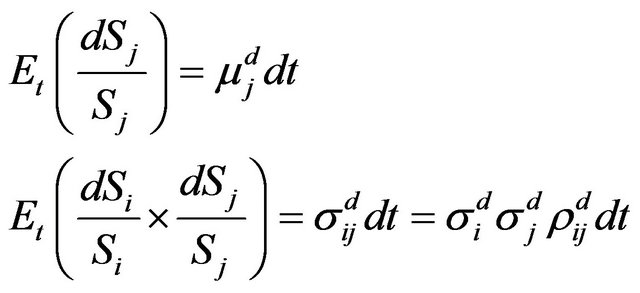
where r is the constant continuous riskless rate of return. Moreover, there are N risky assets in the economy. Each of them follows a pure-diffusion process given by the well known expression,
 (2)
(2)
where  is the price of asset j,
  is a Brownian motion,
  is the drift, and
  is the volatility, and superscript d highlights the pure diffusion character of the process. We denote by
  the NxN covariance matrix of the diffusion components where the typical component of this matrix is
  with
with  being the correlation between the Brownian shocks
  and
and . In matrix notation,
  is the N-vector of expected returns,
  , where
  is the diagonal matrix of volatilities, and
  is the symmetric matrix of correlations.
We next allow for unexpected rare systemic events by introducing a jump to the process given in Equation (2). Following [6], we assume that the jump arrives at the same time across all equity portfolios, and that all portfolios jump in the same direction. Then,
 (3)
(3)
where Q is a Poisson process with common constant intensity , and
, and  is the random jump magnitude that generates the percentage change in the price of asset j if the Poisson event is observed. It is important to note that the arrival of jumps occur at the same time for all equity portfolios. We assume that the Brownian shock, the Poisson jump, and the jump amplitude
  are independent, and that
  has a Normal distribution
  with constant mean
  and variance
 . Therefore, the distribution of the jump size is allowed to be different for each portfolio, although all jumps arrive at the same time.
We define  and
and  as the drift N-vector and the NxN covariance matrix of the diffusion components of Equation (3) respectively. It must be noted that they are now the drift and the covariance matrix of the diffusion components when there are jumps in the return process. In this case, we also have an additional drift,
  , and an additional covariance matrix,
  , from the jump components of the process. Given that we select the parameters of the jump-diffusion process in Equation (3) such that the first two moments for this process match exactly the first two moments of the pure diffusion process in Equation (2), it must be the case that,
 (4)
(4)
2.2. Portfolio Allocation
Our representative investor maximizes the expected power utility defined on terminal wealth,  , given by the well known expression
 , where
  is the constant relative risk aversion coefficient. We first briefly describe the optimal portfolio weights using the pure-diffusion process given in Equation (2). Denoting the vector of the proportions of wealth invested in risky equity portfolios by
 , the optimal portfolio problem at t is
 (5)
(5)
subject to the dynamic budget constraint
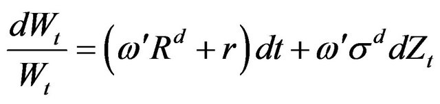 (6)
(6)
where  is the N-vector of excess returns,
  is the diagonal matrix of volatilities,
  is the vector of diffusion shocks, and
  is an N-vector of ones. The solution is the vector of portfolio weights obtained in [9] corresponding to the standard diffusion process of Equation (2),
 (7)
(7)
When the process includes a jump component as in Equation (3), the dynamics of wealth for the initial wealth  can be written as
 (8)
(8)
where  is the N-vector of excess returns,
  is the diagonal matrix of volatilities,
  is the vector of diffusion shocks under a jump-diffusion process, and
  is the vector of random jump amplitudes for the N equity portfolios.
One can employ stochastic dynamic programming to solve for the optimal weights,
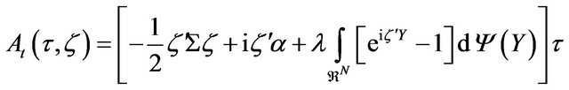
 where in this equation, we can use the generalized jumpdiffusion Ito´s lemma to calculate the differential of the value function,
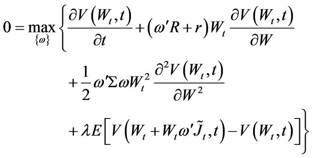
 .4 Then, the Hamilton-Jacobi-Bellman equation is
 (9)
(9)
The impact of the jumps in the return process is given by the last term of Equation (9). This term employs the fact that , and the assumption of indepen dence of the Poisson jump and the jump amplitude except for the fact that the jump size is conditional on the Poisson event happening. As usual in this type of problems, one can guess the solution to the value function as having the following form:
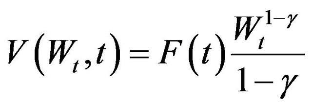 (10)
(10)
Replacing this solution into the Hamilton-Jacobi-Bellman equation we get:
 (11)
(11)
By differentiating with respect to  we obtain the optimal weights with systemic jumps as the solution for each time t to the system of N nonlinear equations which must be solved numerically:
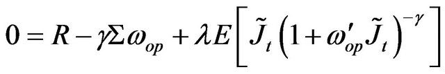 (12)
(12)
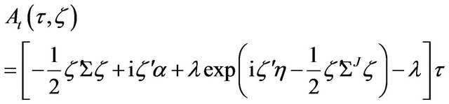
It should be pointed out that if we replace Equation (10) into the Hamilton-Jacobi-Bellman equation and evaluate at  we obtain:
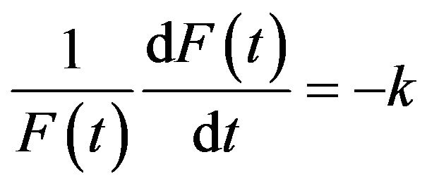 where,

We next employ the boundary condition  to obtain,
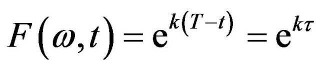
Therefore, the value function is given by the expression
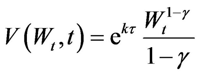 (13)
(13)
2.3. Certainty Equivalent Cost
As an additional analysis of the effects of ignoring systemic risk on asset allocation, we can also calculate the certainty equivalent cost (CEQ hereafter) of following an allocation strategy that ignores the simultaneous jumps occurred in the data. The CEQ gives the additional amount in U.S dollars that must be added to match the expected utility of terminal wealth under the pure-diffusion suboptimal allocation to that under the optimal strategy with the jump-diffusion process of equity returns. In other words, as in [6], we calculate CEQ as the marginal amount of money that equalizes pure-diffusion expected utility with the jump-diffusion expected utility. The compensating CEQ wealth is therefore computed by equating the following expressions:
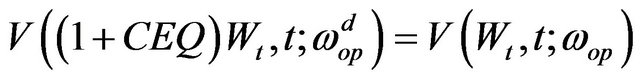 (14)
(14)
Then, using Equation (10) we have that
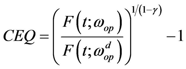 (15)
(15)
3. The Estimation Procedure to Analyze the Effects of Systemic Risk
Let us start again with the pure-diffusion case given by Equation (2). The parameters to be estimated are  where
where  and
and  are the N-vector of expected returns and the NxN covariance matrix of the diffusion components. The moment conditions for individual equity portfolios are given by
 (16)
(16)
This implies that moment conditions  can be estimated directly from the means and the covariance of the actual sample series available.
On the other hand, to derive the four unconditional moments of the jump-diffusion process given in Equation (3), we follow [6] to identify the characteristic function which can be differentiated to obtain the moments of the equity portfolio returns process. We next present a detailed exposition of the procedure employed to obtain the moments under the systemic-jump-diffusion process.
3.1. The Characteristic Function
We first write the previous process in log returns with . It is well known that the pure-diffusion process in Equation (2) becomes
 , (17)
where . As before, the model in matrix notation is
 , where
  is the N-vector of expected returns, and
  is the diagonal matrix of volatilities. On the other hand, the jump-diffusion return process can be written as
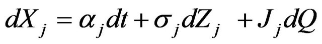 (18)
(18)
where . Hence, in matrix notation, the continuously compounded asset return vector for the jump-diffusion model satisfies the following stochastic differential equation
 , where
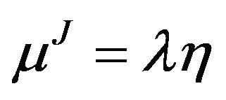
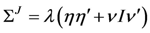
  is the N-vector of expected returns,
  is the diagonal matrix of volatilities for the jump-diffusion case, and J is the N-vector of jump amplitudes. The N-vector of the average size of the jumps amplitude is denoted by
 , while the diagonal variance matrix of the size of the jumps is denoted by
 .
.
As mentioned before, the theoretical moments for the jump-diffusion process are calculated using the characteristic function which in turn can be derived from the Kolmogorov theorem. We formally work in a probability space  where, in the jump-diffusion case, both the process Q and the Brownian motion Z generate the filtration
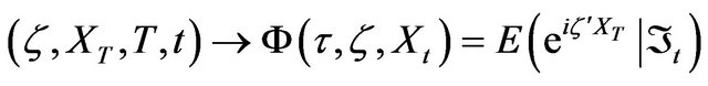
 . The conditional characteristic function of the process X conditioned on
  is defined as the expected value of
 , where
  is the argument of the characteristic function,
  , given by
 (19)
(19)
where .
.
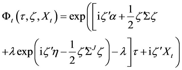
From the process X, we know that  and
and  are constant on X. Therefore, under some technical regularity conditions discussed in [10], the conditional characteristic function has an exponential affine form given by
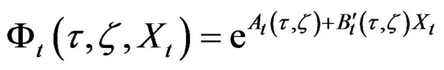 (20)
(20)
According to the Feynman-Kac theorem, the conditional characteristic function is the solution to
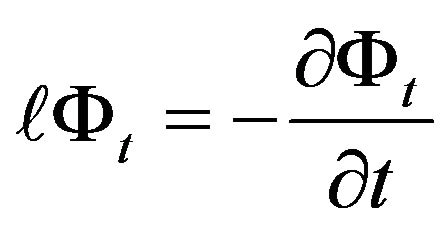 , (21)
where  is the infinitesimal generator for the jumpdiffusion process X given by
 , (22)
where, as already pointed out,  is the jump amplitude Normal distribution. The boundary condition for the differential equation is the value of the conditional characteristic function at the equity portfolio horizon
 . Thus, from Equation (20), it must be the case that
  and
and . In order to find out the expressions for the functions
  and
and , Equation (20) is replaced into Equation (22) to obtain
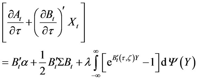 , (23)
where .
.
Thus, the two ordinary differential equations are
 (24)
(24)
The second expression in Equation (24) implies that B does not depend on . Thus, using the boundary condition, we obtain
 . We now replace B in the first equation, we integrate, and we use the remaining boundary condition to get
 (25)
(25)
The integral in the right hand side of Equation (25) can be recognized as the jump amplitude’s characteristic function, given that the random variable J follows a Normal distribution:
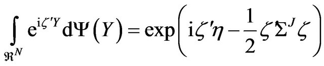
Therefore,
 , (26)
and, finally, the characteristic function is given by
 (27)
(27)
3.2. Unconditional Moments
Using the characteristic function one can derive the K comoments throughout the following expression:
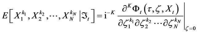 , (28)
where . The gradient and the Hessian,
 and
and  are used to find the first and second moments respectively. For the one-period investment horizon,
  , and using the conversion from the noncentral to central moments we obtain the mean, covariance, coskewness, and excess kurtosis:5
 (29)
(29)
 (30)
(30)
 (31)
(31)
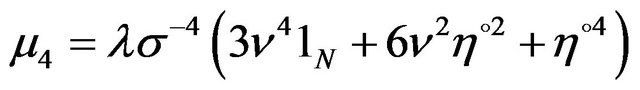 (32)
(32)
In the expressions above, I is the NxN matrix of ones, and  denotes the N-times element-by-element multiplication. It should be noted that
  and
and  are Nvectors, and
  and
and  are NxN matrices.
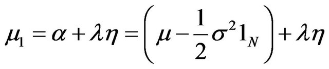
If we now compare the mean and covariance for the jump-diffusion process above with those for the purediffusion processes for , we observe that
 (33)
(33)
 (34)
(34)
Then, the diffusion moments of the jump-diffusion process are retrieved using the expressions in Equation (4) as:
 (35)
(35)
 (36)
(36)
From the moment conditions in Equations (29)-(32) the parameters to be estimated are . For the universe of N assets there are N jump amplitude means and N jump amplitude volatilities. This represents 2N+1 parameters to be estimated including the Poisson intensity
 . On the other hand, there are
  co-skewness moments and N excess kurtosis moments for a total of
  moment conditions to be employed in the generalized method of moment (GMM) estimation procedure.
3.3. Sampling Moments
The sampling mean and co-moments of a variable X with respect to variable Y are:
for  and
and , where
  is the adjustment term for the unbiasedness correction.
4. Optimal Allocation for Value and Growth Portfolios with Systemic Risk: Empirical Results
We estimate the model using 3 portfolios from the 10 monthly book-to-market sorted portfolios taken from Kenneth French’s web page. Portfolio 1 contains the companies with low book-to-market, while portfolio 10 includes assets with high book-to-market. We refer to portfolio 1 as the growth portfolio, and portfolio 10 as the value portfolio. We also employ portfolio 5 denoted as the intermediate portfolio. In order to pay special attention to these characteristics we use the equallyweighted scheme of the individual stocks rather than the more popular value-weighted portfolios. This weighting approach also amplifies the value effect anomaly.
4.1. Parameter Estimates for the Jump-Diffusion Return Process
Table 1 reports the descriptive statistics of the three monthly Fama-French book-to-market portfolios for the full sample period from January 1982 to October 2010
Table 1. Descriptive statistics for the fama-french growth and value portfolios. (a) Moments of the monthly returnsa; (b) Correlation coefficientsb.
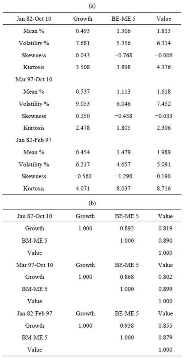
aPanel A of this table reports the first four moments of the monthly returns for the growth and value portfolios constructed by Fama-French using their ten book-to-market sorted portfolios, where the first portfolio is the growth portfolio, portfolio BE-ME 5 is the intermediate portfolio, and the last portfolio is the value portfolio. The data for the full period goes from January 1982 to October 2010, while the sub-periods contain data from January 1982 to February 1997 and from March 1998 to October 2010. bPanel B of the table gives the correlation coefficients among the monthly returns for the growth, intermediate, and value portfolios.
and two sub-periods from January 1982 to February 1997, and from March 1997 to October 2010. Both sub-periods contain episodes with large negative shocks. The first sub-period includes the market crash of October 1987, the Gulf War I in August 1990, and the Mexican crisis in December 1994. On other hand, the second sub-period contains the Asian crisis of July 1997, the Russian crisis of August 1998, the bursting of the dot.com bubble, the terrorist attack of September 2001, the outbreak of the Gulf War II in March 2003, the beginning of the subprime crisis, and the Lehmann Brothers default in September 2008.
Panel A of Table 1 shows that the use of the equallyweighted growth and value portfolios leads to an impressive value premium of 15.8% on annual basis for the full sample period. Moreover, the value premium is 13.0% and 18.4% for the second and first sub-periods respecttively. As expected, the annualized volatility of the growth portfolio is higher than the corresponding volatility of the value portfolio is all three sample periods. On annual basis, the growth volatility premium is 4.7% for the full period, and 5.6% and 3.9% for the second and first sub-periods respectively. Indeed, the growth portfolio seems to be riskier than the value portfolio. The problem is, of course, the enormous average return of the value portfolio.
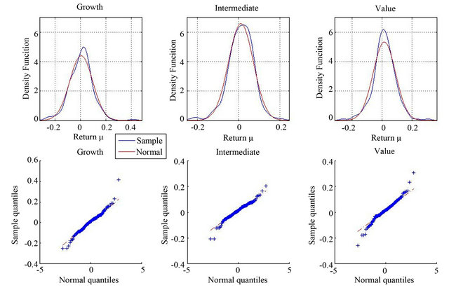
The third and fourth moments of both portfolios also present an interesting behaviour. For the full period, the growth portfolio has positive skewness, while the value portfolio has a slightly negative skewness. Moreover, growth stocks have lower kurtosis than the value portfolio. The overall behaviour is the consequence of two very different sub-periods. From 1997 to 2010, the value portfolio has negative skewness, and, on the contrary, growth stocks have positive skewness. The excess kurtosis is similar for both portfolios. However, from 1982 to 1997, we report a very high negative skewness for the growth portfolio, and a positive skewness for value stocks. Similarly, the behaviour of excess kurtosis is also surprising. Value stocks present a much higher kurtosis than the growth portfolio. The changes observed in both skewness and kurtosis from one sub-period to the other for growth and value portfolios are striking and deserve further attention. For completeness, Figure 1 shows the density functions for both sub-periods of the growth, intermediate and value portfolios, and the QQ plots to assess the deviations of their returns from the Normal distribution.
Panel B of Table 1 reports the correlation coefficients among the three book-to-market portfolios. The results show that from 1997 to 2010 the value and growth portfolios are less correlated than in the previous sub-period.
Panel A of Table 2 contains the parameter estimates obtained by the generalized method of moments with the
Table 2. Parameter estimates for the returns processes with jumps. (a) Parameter estimates for the jump processa; (b) Comparison between higher order sample moments of returns and the jumps process theoretical higher order momentsb.
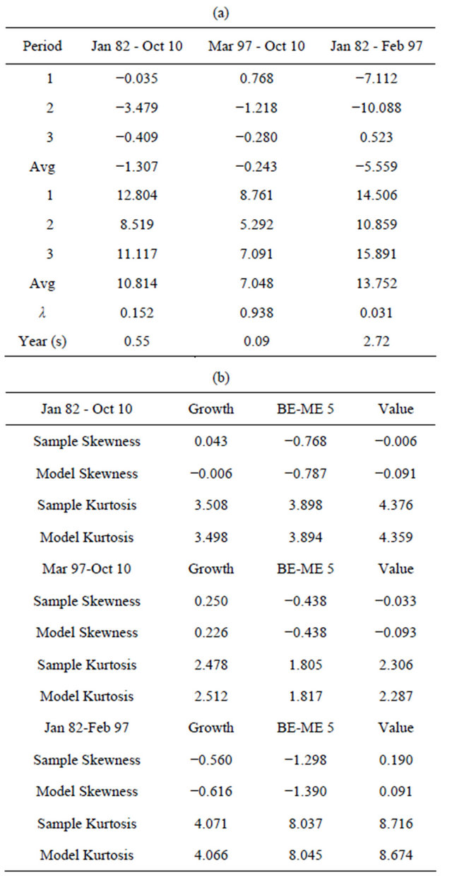
aPanel A of this table reports estimates of the parameter for the jump-diffusion portfolio returns obtained by minimizing the square of the difference between the theoretical moment conditions and the moments implied by the data. , for j = 1, 2, 3, refers to the mean of the jump size for the growth, intermediate, and value portfolios respectively.
 , for j = 1, 2, 3, is the volatility of the jump size for the growth, intermediate, and value portfolios respectively. These estimates are given in percentage terms. Avg gives the average magnitude of the average and volatility jump sizes across portfolios,
  represents the frequency of the jumps, and Year (s) is the number of years necessary to observe a jump according to the jump-diffusion process. bPanel B contains the reconstructed moments that are obtained by substituting the parameter estimates in the theoretical model, and the sample moments.
 (a)
(a) (b)
(b)
Figure 1. Density functions and QQ plots; (a) March 1997-October 2010; (b) January 1982-February 1997.
identity matrix using Equations (29)-(32). The estimated value for  of 0.152 for the full sample period implies that on average the chance of a simultaneous jump in any month across book-to-market portfolios is about 15%, or one jump is expected every 6.6 months or, equivalently, 0.55 years. The average size of the jump across three portfolios is −1.307, and it seems much higher (in absolute value) for the value portfolio than for the growth stocks. Although, the intermediate portfolio has the highest average size of the jump, the volatilities of the size of the jumps are higher for the extreme growth and value portfolios.
As before, the more interesting results come from the changing behavior of the growth and value stocks across sub-periods. The estimated value for  of 0.938 from 1997 to 2010 implies that on average the chance of a simultaneous jump in any month across book-to-market portfolios is almost 94%, or one jump is expected every 1.1 months or 0.09 years. Hence, the frequency of simultaneous jumps in the last sub-periods is extremely high. However, during this sub-period, the average size of the jump is −0.243 which is a relatively low relative to the estimate for the full sample period. This relatively small average size is partly due to the compensation between the positive average size for growth stocks, and the negative average size for value stocks. Hence, form 1997 to 2010, growth stocks have on average positive jumps, while value stocks present on average negative jumps. At the same time, the volatility of the size of the jumps seems to be lower than the volatility for the full sample period. The crisis episodes of the last decade or so, seems to affect much more negatively value than growth stocks. This is clearly consistent with the negative (positive) skewness for the value (growth) stocks from 1997 to 2010. The economic implication is that value stocks seem to be more pro-cyclical than growth stocks.
Once again, the estimation results are very different for the first sub-period from 1982 to 1997. The estimated value for  of 0.031 from 1982 to 1997 implies that, on average, the chance of a simultaneous jump in any month across book-to-market portfolios is about 3%, or one jump is expected every 32.3 months or 2.7 years. Hence, the frequency of simultaneous jumps in the first subperiod is much lower than in the most recent sub-period. This is, by itself, a relevant result. During the last fourteen years, there seems to be many more systemic jump episodes than during the previous fifteen years. Somehow surprisingly, however, the average size of the jump from 1982 to 1997 is strongly negative and much larger in absolute value than during the last sub-period. Also, the volatility of the size of the jumps is much larger than the volatility reported from 1997 to 2010. Interestingly, the average size of the jump is positive (negative) for value (growth) stocks which are precisely the opposite reported from 1997 to 2010. Again, this is consistent with the negative (positive) skewness for the growth (value) portfolio shown in Table 1. It is also important to point out that it is precisely in this sub-period when the value premium is as high as 18.4% on annual basis. The jumps of the first sub-period are therefore much less frequent but of larger magnitude than the jumps observed from 1997 to 2010. The relatively few but larger jumps affect more negatively growth stocks, while very frequent although smaller jumps impact more negatively value stocks. Again, it should be recalled that the value premium is much larger from 1982 to 1997 than from 1997 to 2010.
Panel B of Table 2 compares the reconstructed moments that are obtained by substituting the parameter estimates in the theoretical jump-diffusion model and the sample moments. As before, the comparison exercise is performed for each of the three sample periods. Overall, the jump-diffusion model captures very well the sample excess kurtosis for all time periods and portfolios. However, the model seems to have more problems fitting the magnitudes of the asymmetry of the distribution of returns. This is especially true for the value portfolio, where the theoretical process overstates the magnitude of skewness. This result comes basically from the bad performance of the model capturing the skewness of value stocks from 1997 to 2010. The jump-diffusion process generates much more negative skewness than the one observed in the data.
4.2. Portfolio Weights
We want to solve numerically Equation (12) to obtain the optimal weights when the return process follows the jump-diffusion model of Equation (3). The parameters we employ for the return process are those reported in Panel A of Table 2. We also assume that the annualized risk-free rate is equal to 6%, and we solve for optimal weights assuming 10 alternative values of the relative risk aversion coefficient. As the benchmark case, we use the pure-diffusion model where the optimal weights are given by the well known expression in Equation (7).
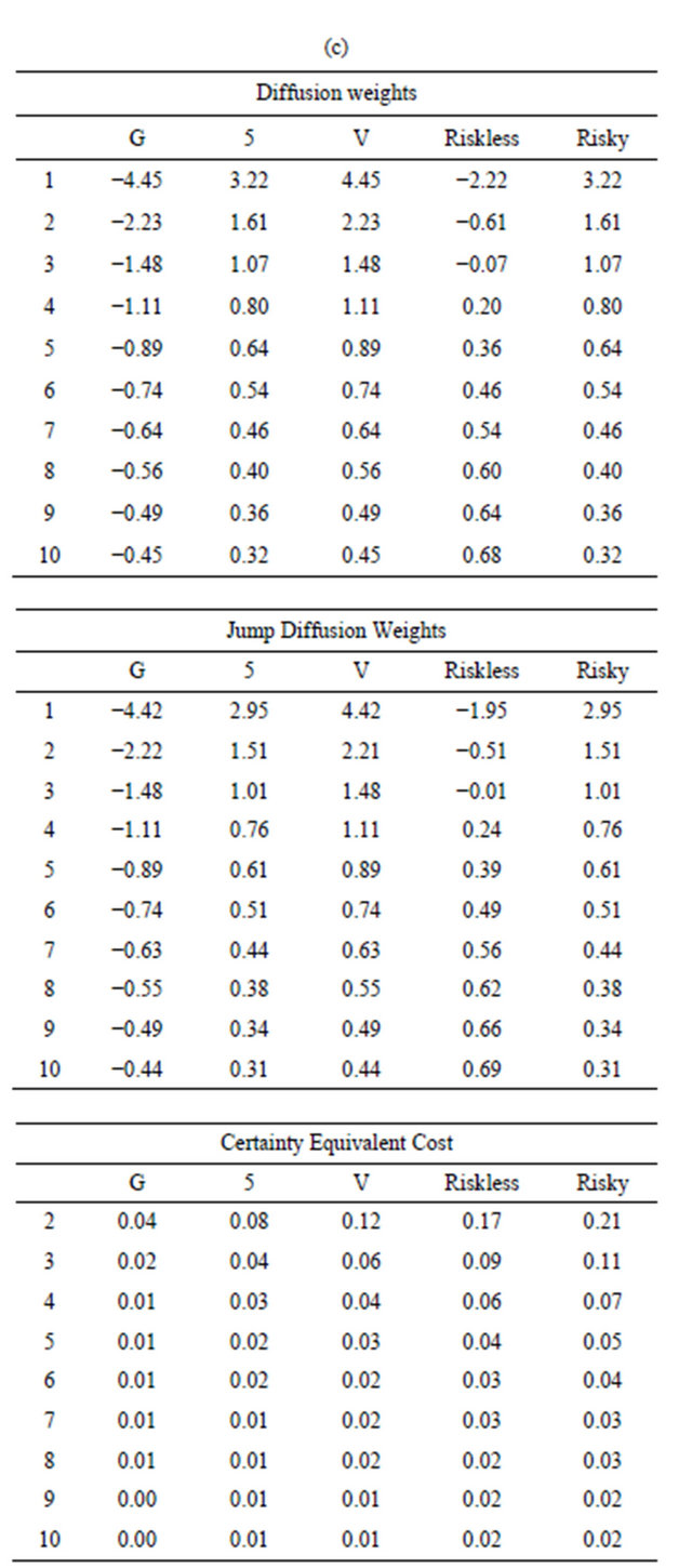
Panel A of Table 3 contains the equity portfolio allocation results for the benchmark case, while Panel B reports the results for the jump-diffusion model. The results show that, independently of the sample period employed and the level of risk aversion, value stocks receive a higher investment proportion of funds than growth stocks. The optimal allocation implies in all cases to go long in the value portfolio and short on the growth portfolio. This is also true whether we recognize simultaneous jumps across assets or not. This is, of course, what a zero-cost investment on the HML portfolio in [11] precisely does. Surprisingly, for the full sample period, the intermediate book-to-market portfolio dominates the value portfolio due to the large weights this portfolio gets from 1982 to 1997. For this first sub-period, it must be pointed out that, when we incorporate jumps, the value portfolio indeed gets more proportion of wealth than the intermediate portfolio but only for the most levered position. It is interesting to observe the important impact that jumps have in this case for the nonconservative investor. The proportion invested in the intermediate assets decreases from 28.7% without jumps to 17.4% with jumps, while the same proportions go from 14.0% to 18.5% for the value portfolio.
Finally, the value portfolio dominates the investment in the risky component of the optimal asset allocation for the 1997 to 2010 sub-period independently of recognizeing jumps or not.
From Panel C of Table 3, where we report the differences in weights between the benchmark case and the jump-diffusion model, we observe that, for the overall sample period, the recognition of jumps diminishes the differences in the sense of increasing the long position on
Table 3. Portfolio Weights. (a) Diffusion Weightsa; (b) Jump-diffusion (Systemic) Weightsb; (c) Diffusion-Jump Weight Differencesc.

aPanel A of this table gives the portfolio weights for an investor who selects investments in three equity portfolios (growth, intermediate, value) and the riskless asset to maximize expected power utility of terminal wealth with constant relative risk aversion. The investor optimizes expected utility ignoring systemic jumps and assumes a pure diffusion process for portfolio returns.  is the relative risk aversion coefficient, G, 5, and V indicate the growth, intermediate portfolio, and value portfolios respectively. Risky is the total weight given to all three equity portfolios. bPanel B reports the optimal weights when the investor recognized systemic jumps. cPanel C contains the differences between the optimal weights for pure diffusion and the weights for the jump-diffusion process.
the value portfolio while, at the same, it suggests not short-selling as much on the growth portfolio.6 The recognition of jumps implies to put relatively fewer funds in the risky portfolio for all levels of risk aversion, although this seems to be especially the case for the nonconservative investors and, therefore, for the most levered positions. However, the main point is that the value portfolio gets more weights for all . At the end, at least from 1982 to 2010, the use of systemic jumps in the optimal allocation of funds, increases the proportion of value stocks, reduces the amount of short-selling in the growth stocks, and diminishes the proportion of funds invested in the intermediate portfolio.
As in other cases, the results of the full sample period seem to be the consequences of two different sub-periods. The effects of jumps from 1997 to 2010 are, to all effects, negligible. The differences of optimal weights between the benchmark case and the jump-diffusion model are therefore basically zero except, if anything, for the highly levered position. The main effects of jumps come from the first sub-period. From 1982 to 1997, there were very few jumps but with a relatively very large average size. In fact, the average jump size for the value portfolio is positive, which makes the proportion of funds invested in value to increase importantly and, especially, for the most levered portfolios. These effects can be seen directly from Panel C of Table 3 and they are also reflected in Figure 2. By recognizing systemic jumps, optimal asset allocation increases significantly for value stocks and for all levels of risk aversion, although more for the less conservative more levered case. At the same time, jumps reduce considerably the proportion invested in the intermediate portfolio. As a consequence of recognizing jumps, there is also a reduction in the short-selling proportions of growth stocks.
The same conclusion is obtained by the results shown in Table 4. We report the percentages of the growth, intermediate, and value portfolios in the total proportion invested in risky assets. We observe that the spread between the proportions invested in value and growth assets is higher in the first than in the second sub-period. It is also the case, that the spread in the first sub-period is particularly important for the most levered portfolios, although the relevance of risk aversion is negligible in the last sub-period.
We may conclude that systemic jumps across portfolios seem to be important for asset allocation as long as the average magnitude of the jumps is large enough. From the point of view of asset allocation, it is therefore more important the amplitude than the frequency of the
Table 4. Composition of the Risky Portfolios. (a) Jumpdiffusion (Systemic) Weightsa; (b) Diffusion Weightsb.
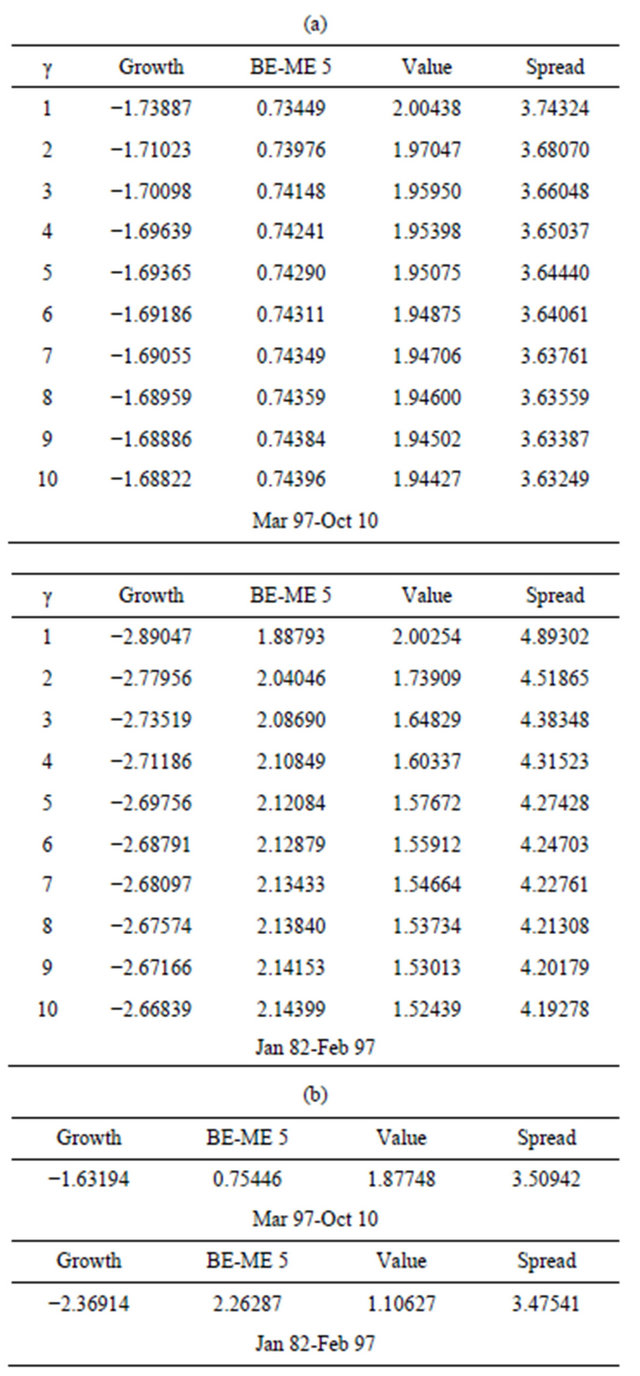
aPanel A of this table contains the composition of the risky portfolios for alternative levels of relative risk aversion, which is obtained by dividing the weight for each portfolio by the total amount invested in risky portfolios. It assumes the jump-diffusion process. bPanel B contains the same results assuming the pure diffusion process. It should be noted that the weights do not depend on the level of relative risk aversion when the simple diffusion process is employed in the estimation.
jumps. In our specific sample, jumps turn out to be relevant for value stocks given the combination of a large and positive average jump size. Jumps also seems to favor value stocks even with a negative average size jump as in the full sample period, but this is relatively less important and, in any case, the possible effects are just concentrated in highly levered portfolios.
4.3. Certainty Equivalent Costs
We next analyze the effect on utility of the optimal portfolio strategy that recognizes the occurrence of systemic jumps across book-to-market assets relative to the strategy that ignores these simultaneous jumps. We employ the CEQ given in Equation (15) that calculates the additional wealth per $1000 of investment needed to raise the expected utility of terminal wealth under the nonoptimal portfolio strategy to that under the optimal investment strategy. We consider the effects for investment horizons of 1 to 5 years and for levels of risk aversion of 2 to 10.
Table 5 reports the results. As before, the effects of frequent but relatively small jumps observed from 1997 to 2010 is negligible. Even the U.S. dollar consequences of the nonoptimal strategy over the full sample period are very small. For highly risk-taken investors and over a 5 years horizon, the cost of ignoring jumps is only about $2.00.
All the relevant effects come, once again, from the 1982 to 1997 sub-period in which the average size jump seems to be high enough to impact the portfolio allocation of equity portfolios. As we observe, the CEQ decreases as risk aversion increases. This suggests that, as he becomes more risk averse, the investor holds a smaller proportion of his wealth in risky portfolios and, therefore, both the exposure to simultaneous jumps and the effects
 (a)
(a) (b)
(b)
Figure 2. Portfolio weights and relative risk aversion. (a) Pure-diffusion process; (b) Jump-diffusion process; This figure shows the portfolio weights for the growth, intermediate and value Fama-French portfolios for alternative levels of relative risk aversion. Panel A contains the weights for the pure-diffusion process, while Panel B gives the weights for the jump-diffusion process. The first figure of each panel corresponds to the last sample period from March 1997 to October 2010, and the second figure of each panel corresponds to the first sample period from January 1982 to February 1997.
on CEQ are smaller. However, when the investor is willing to accept higher risks, his optimal portfolio becomes much more levered to buy additional risky assets. Then, the consequences of ignoring systemic jumps should be higher. This is exactly what we observe from Table 5
Table 5. Certainty equivalent cost of ignoring systemic jumpsa.
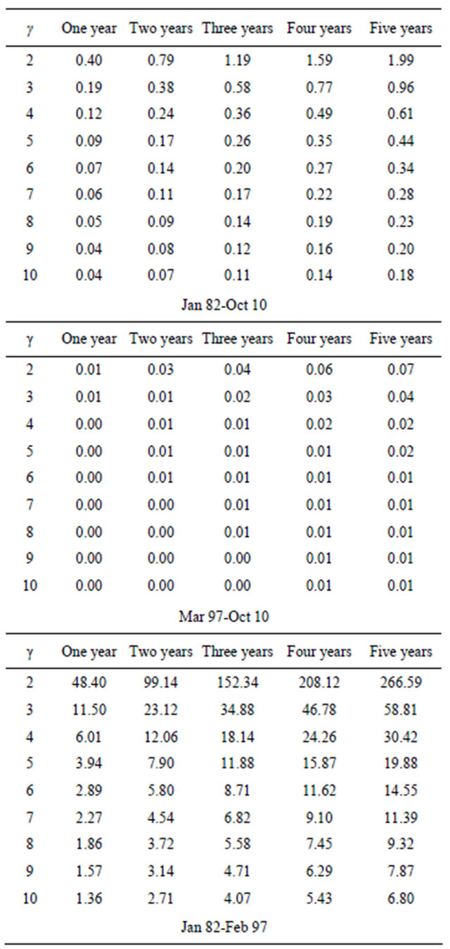
aThis table reports the certainty equivalent costs (CEQ) of ignoring systemic jumps calculated as the additional wealth per $1,000 of investment needed to raise the expected utility of terminal wealth under the suboptimal portfolio strategy to that under the optimal investment strategy. The table contains the CEQ for investment horizons of 1 to 5 years, and for levels of relative risk aversion  from 2 to 10.
and Figure 3. For highly levered portfolios, the CEQ goes from $48.40 for a 1-year horizon to $266.50 for the longest horizon per $1000 of investment. It should not be surprising that the higher the leverage position of an investment is, the higher the impact of jumps on portfolio strategies. It should be recognized however, that the dollar effects diminish very rapidly as the investor becomes more risk averse. For , even for the longest horizon of 5 years, the CEQ is $30.42 per $1000 which does not seem to be substantial.
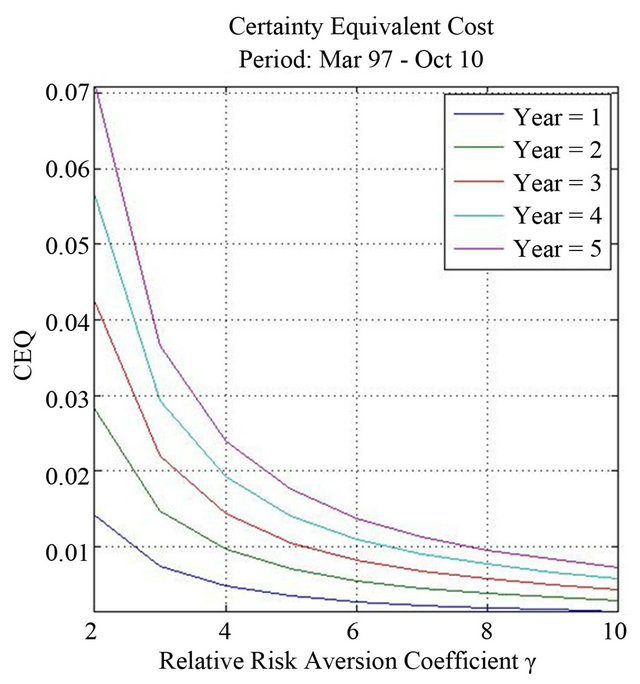
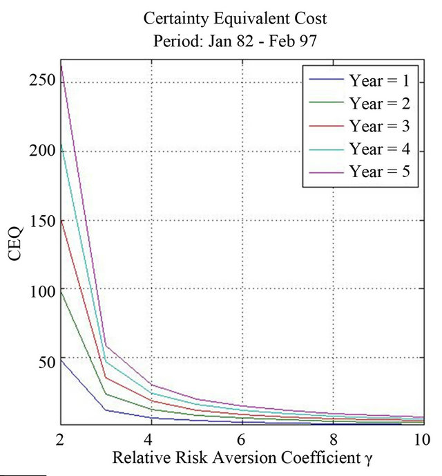
Figure 3. Certainty equivalent cost of ignoring systemic jumps. This figure shows the certainty equivalent costs (CEQ) of ignoring systemic jumps calculated as the additional wealth per $1,000 of investment needed to raise the expected utility of terminal wealth under the suboptimal portfolio strategy to that under the optimal investment strategy. The figure contains the CEQ for investment horizons of 1 to 5 years, and for levels of relative risk aversion  from 2 to 10. The first figure corresponds to the last sample period from March 1997 to October 2010, and the second figure of each panel corresponds to the first sample period from January 1982 to February 1997.
4.4. Sample Average Riskless Rate
In the previous discussion, we impose a 0.5% monthly riskless rate for the full sample period and for both subperiods. Although this is a reasonable riskless rate for the first sub-period, it may be too high for the second subperiod. For this reason, we estimate again the model from 1997 to 2010 imposing the actual average riskless rate of 0.5% per month or 3% per year. It must be noted that the interest rate affects the parameter estimates and, therefore, it may have consequences for the general conclusions about the optimal portfolio allocation during the second sub-period.
Table 6 reports the results affected by the riskless rate. The empirical evidence is almost identical to the evidence contained in Tables 2, 3 and 5. The average size of jumps is even slightly lower, and the frequency of the jumps is now 1.231 relative to the previous estimate of 0.938. Thus, the frequency of the simultaneous jumps is higher than the one reported in Table 2. Once again, this sub-period is characterized by many jumps of small average amplitude. The effects of jumps on the portfolio weights and on the cost of ignoring jumps are very similar to the previously reported results. As expected, given that now the risk-free investment offers a lower rate, the optimal amount of the risky portfolios is higher with respect to the allocation shown in previous tables. However, the effects about the distribution of resources among book-to-market portfolios with or without jumps are negligible. All our previous conclusions remain the same
Table 6. Jump diffusion parameter and weight estimates March 1997-October 2010 for the sample average annualized riskless rate of 3%. (a) Parameter estimates for the jump processa; (b) Comparison between higher order sample moments of returns and the jumps process theoretical higher order momentsb; (c) Diffusion weights, jump-diffusion weights and certainty equivalent costs (CEQ)c.
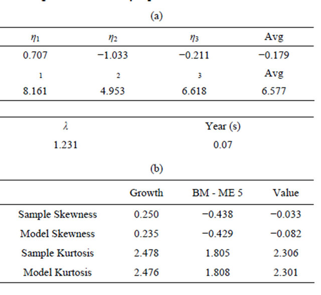
aPanel A reports the estimates of the parameters for the jump-diffusion portfolio returns for an annualized riskless rate of 3%. bPanel B contains the reconstructed moments and the sample moments. cPanel C these tables gives the portfolio weights for an investor who ignoring systemic jumps, the optimal weights when the investor recognized systemic jumps and the certainty equivalent costs (CEQ) of ignoring systemic jumps calculated as the additional wealth per $1,000 of investment needed to raise the expected utility of terminal wealth under the suboptimal portfolio strategy to that under the optimal investment strategy.
even with a much lower riskless rate.
4.5. Specification Tests with a Pre-Specified Weighting Matrix
Up to now, the statistical performance of the model has been very informal. Intentionally, our discussion has been based mainly on economic intuition rather than statistical formality. We finally want to test the overall fit of the model. The test-statistic is the GMM test of overidentification restrictions.
We denote by  the K-vector of moment conditions containing the pricing errors generated by the jump-diffusion model at time t, and by
  the set of parameters to be estimated. The corresponding sample averages are denoted by
 . Then, the GMM estimator procedure minimizes the quadratic form
 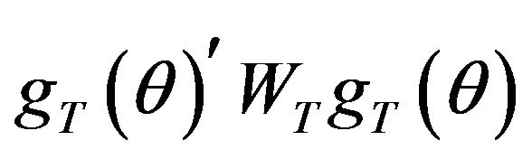 where
where  is a weighting squared matrix. The evaluation of the model performance is carried out by testing the null hypothesis
 with
with  where the weighting matrix, W, is in our case the identity matrix. If the weighting matrix is optimal,
  is asymptotically distributed as a Chi-square with K–P–1 degrees of freedom, where P is the number of parameters. However, for any other weighting matrix (including the identity matrix), the distribution of the test statistic is unknown. Reference
[12] shows that, in this case,  is asymptotically distributed as a weighted sum of K–P–1 independent Chi-squares random variables with one degree of freedom. That is
 (37)
(37)
where , for
, for , are the positive eigenvalues of the following matrix:
 in which
  means the upper-triangular matrix from the Choleski decomposition of X, and
  is a K-dimensional identity matrix. Moreover,
  and
and  are given by,

Therefore, in order to test the different models we estimate, we proceed in the following way. First, we estimate the matrix  and compute its nonzero K–P–1 eigenvalues. Second, we generate
 ,
,  ,
,  , independent random draws from a
  distribution. For each h,
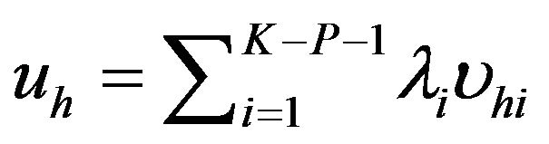 is computed. Then we compute the number of cases for which
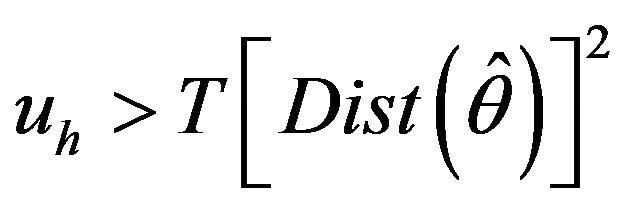 . Let p denote the percentage of this number. We repeat this procedure 1000 times. Finally, the p-value for the specification test of the model is the average of the p values for the 1000 replications.
It turns out that we are not able to reject the jumpdiffusion model in any of the alternative sample periods employed in the estimation. The p-values for the full sample period, the first sub-period, and the second subperiod are 0.257, 0.103, and 0.676 respectively. These results suggest that the jump-diffusion model fits the actual data better from 1997 to 2010 than from 1982 to 1997. This is the case despite the poor reconstruction of the actual skewness for the value portfolio from 1997 to 2010.
4.6. Conclusions
Given the tendency of globalization and increasing integration of financial markets, it is generally accepted that equity portfolios of different characteristics and also international equities are characterized by simultaneous jumps. We investigate the effects of these jumps on optimal portfolio allocation using value and growth stocks and two different sub-periods. It seems that the effects of systemic jumps may be potentially substantial as long as market equity returns experiment very large average (negative) sizes. However, it does not seem to be relevant that stock markets experience very frequent jumps if they are not large enough to impact the most levered portfolios. All potentially relevant effects are concentrated in portfolios financed with a considerable amount of leverage. In fact, for conservative investors with low leverage positions the potential effects of systemic jumps on the optimal allocation of resources are not substantial even under large average size jumps. Finally, the value premium is particularly high when the average size of the jumps of value stocks is positive, large and relatively infrequent, while the average size of growth stocks is also very large but negative. It seems therefore plausible to conclude that the magnitude of the value premium is closely related to the characteristics of the jumps experienced by value and growth stocks.
5. Acknowledgements
Gonzalo Rubio acknowledges financial support from Ministry of Economía and Competitividad grant MEC ECO2012-34268, and the Prometeo Program of the Generalitat Valenciana under project PROMETEO/208/106, and Banco de Santander-Copernicus/104. A preliminary version of this paper was presented at the XIX Foro de Finanzas at the University of Granada, Spain. The authors thank participants for helpful suggestions. We especially thank the constructive and useful comments of Santiago Forte and Belén Nieto.
REFERENCES
- L. Zhang, “The Value Premium,” Journal of Finance, Vol. 60, No. 1, 2005, pp. 67-103. doi:10.1111/j.1540-6261.2005.00725.x
- M. Yogo, “A Consumption-Based Explanation of Expected Stock Returns,” Journal of Finance, Vol. 61, No. 2, 2006, pp. 539-580. doi:10.1111/j.1540-6261.2006.00848.x
- F. Belo, C. Xue and L. Zhang, “The Value Spread: A Puzzle,” Working Paper, Ohio State University, 2010.
- L. Chen and L. Zhang, “A Better Three-Factor Model that Explains More Anomalies,” Journal of Finance, Vol. 65, No. 2, 2009, pp. 563-594.
- Squam Lake Report Group, “Fixing the Financial System,” Princeton University Press, New York, 2010.
- S. Das and R. Uppal, “Systemic Risk and International Portfolio Choice,” Journal of Finance, Vol. 59, No. 6, 2004, pp. 2809-2834. doi:10.1111/j.1540-6261.2004.00717.x
- T. Andersen, L. Benzoni and J. Lund, “An Empirical Investigation of Continuous-Time Equity Return Models,” Journal of Finance, Vol. 57, No. 3, 2002, pp. 1239- 1284. doi:10.1111/1540-6261.00460
- A. González, A. Novales and G. Rubio, “Efficient Method of Moments Estimation of Stochastic Volatility and Jumps in European Stock Market Return Indices,” Working Paper, Universidad CEU Cardenal Herrera, and Instituto Complutense de Análisis Económico (ICAE), 2011.
- R. C. Merton, “Lifetime Portfolio Selection under Uncertainty: The Continuous-Time Case,” The Review of Economics and Statistics, Vol. 51, No. 3, 1969, pp. 247-257. doi:10.2307/1926560
- D. Duffie, J. Pan and K. Singleton, “Transform Analysis and Asset Pricing for Affine Jump Diffusions,” Econometrica, Vol. 68, No. 6, 2000, pp. 1343-1376. doi:10.1111/1468-0262.00164
- E. Fama and K. French, “Common Risk Factors in the Returns on Stocks and Bonds,” Journal of Financial Economics, Vol. 33, No. 1, 1993, pp. 3-56. doi:10.1016/0304-405X(93)90023-5
- R. Jagannathan and Z. Wang, “The Conditional CAPM and the Cross-Section of Expected Returns,” Journal of Finance, Vol. 51, No. 1, 1996, pp. 3-53. doi:10.1111/j.1540-6261.1996.tb05201.x
NOTES
1These numbers correspond to the 10 Fama-French monthly portfolios sorted by book-to-market, and using a value-weighted scheme to obtain the portfolio returns. The value premium using an equallyweighted approach is an even much higher 14.0% on annual basis.
2In [1] it is argued that costly reversibility and countercyclical market price of risk cause assets in place to be harder to reduce so they, in fact, become riskier than growth options. A related argument is given in [2] which employs nonseparability between durable and nondurable consumption to show that value stocks are more procyclical than growth stocks. This implies that they perform especially badly during economic downturns. However, recent evidence provided in [3] shows that the q-theory dynamic investment framework fails to explain the value spread. This is the case despite the fact that in [4] it is argued that a simple three-factor model inspired on the q-theory of investment is able to explain anomalies associated with short-term prior returns, financial distress, net stock issues, asset growth, earnings surprises, and some valuation ratios.
3See [5] for a clarifying discussion of these issues.
4Alternatively, we may employ the infinitesimal generator of the jumpdiffusion process in [10].
5A technical appendix is available from the authors upon request. The Appendix derives the unconditional moments using alternative procedures. These derivations extend and complete the mathematical technicalities suggested in [6].
6A negative sign for the value portfolio in Panel C indicates that the recognition of simultaneous jumps makes the investor to allocate more funds in the value portfolio. A negative sign on the growth portfolio implies that the recommendation would be to short-sale growth stocks in less proportion than the case of the pure-diffusion benchmark.