Open Journal of Marine Science
Vol.4 No.1(2014), Article ID:42001,7 pages DOI:10.4236/ojms.2014.41003
Application of Stationary Phase Method to Wind Stress and Breaking Impacts on Ocean Relatively High Waves
Laboratory of Earth’s Atmosphere Physics, Department of Physics, Faculty of Science, University of Yaoundé I, Yaoundé, Cameroon
Email:*cesar.mbane@yahoo.fr
Copyright © 2014 Augustin Daika et al. This is an open access article distributed under the Creative Commons Attribution License, which permits unrestricted use, distribution, and reproduction in any medium, provided the original work is properly cited. In accordance of the Creative Commons Attribution License all Copyrights © 2014 are reserved for SCIRP and the owner of the intellectual property Augustin Daika et al. All Copyright © 2014 are guarded by law and by SCIRP as a guardian.
Received September 25, 2013; revised November 3, 2013; accepted December 6, 2013
KEYWORDS
Wind Stress; Granular Targets; Low Surface Tension; Stationary Phase Method; Stationary Gaussian
ABSTRACT
Wind stress impacts on ocean relatively high waves can be perfectly illustrated by a recurrent phenomenon in the Sahara desert. Indeed, on this area where the surface wind can blow without encountering major obstacle out of the sand dunes, these main targets are gradually eroded and displaced by the wind on dozens of meters. This experience highlights the action of wind on granular targets (clusters of sand or water slides) and motivates studies similar to ours, where we want to simulate impact of wind stress and breaking on the spatio-temporal evolution of the envelope of ocean relatively high waves: Impact which can inappropriately deflect the waves on ships, oil platforms or coastal infrastructures. Euler and Navier-Stokes equations allow a mathematical formulation of the gravity wave motion (ocean waves are considered in our work as a system of water particles which are held together by low surface tension) and wind acts on targets through friction forces or stress. Michel Talon stationary phase method is used to numerically solve the equations that model the impact of wind on a stationary Gaussian.
1. Introduction
Since men have traveled on the oceans, they are impressed by these relatively hostile huge rivers that inspire respect and fear. As evidence of this fear, many legends have always circulated that such stories express the existence of mermaids shipwrecks [1,2], the ghost ships savagely attack ships, or even more recently beliefs about the Bermuda Triangle, where ships disappear inexplicably. Among these legends is that of rogue waves that correspond in many respects to deep water gravity waves [3]. Many accounts of seamen have alluded to walls of water rising for no reason in the middle of the sea and hitting ships with extraordinary violence. These stories were not credible until 1978, when the cargo ship “Munchen” disappeared under mysterious circumstances. This vessel at the forefront of naval technology was heading in the North Atlantic, with no apparent problems until the night of December 12. Given that the weather service recorded no storm that night, it is reasonable to believe that a rogue wave is the only plausible explanation for this shipwreck. In 1980, Philippe Lijour, captain of the tanker “Esso Lanuedoc”, demonstrates the existence of rogue waves with a photo as proof. The existence of rogue waves is now universally recognized [4-9], and many images on the extent of damage caused by these monsters of the ocean are available. However, the physical processes responsible for the formation and spread of the phenomenon and its prediction are not completely understood. Contrary to popular belief, Mbane [10] demonstrated that, the natural phenomena like rogue waves are not just spectacular events accessible to routine observations and satellites images. Rogue waves are a combination of complex physical processes that occur under ideal conditions of temperature and humidity [10]. Numerical computations [11-23] offer tremendous opportunities for approaches of physical phenomena for which analytical solutions are at the present stage of development of mathematics, difficult to obtain. Our previous paper [24] based on application of Benjamin-Feir equations to tornadoes’ rogues waves modulational instability in oceans is an important tool for acquiring information on the Kinematics and thermodynamics of atmosphere processes which trigger deep rivers gravity waves. In this regard, tornadoes can give birth to ocean gravity waves whose size varies depending mainly on depth of depression and sea surface temperature [24]. In the Sahara desert, sand dunes are gradually eroded and displaced by the wind on dozens of meters. This experience highlights the action of wind on granular targets (clusters of sand or water slides) and motivates studies similar to ours, where we want to simulate impact of wind stress and breaking on the spatio-temporal evolution of the envelope of ocean relatively high waves: Impact which can inappropriately deflect the waves on ships, oil platforms or coastal infrastructures. Euler and Navier-Stokes equations allow a mathematical formulation of the gravity wave motion (ocean waves are considered in our work as a system of water particles which are held together by low surface tension) and wind acts on targets through friction forces or stress. Michel Talon stationary phase method is used to numerically solve the equations that model the impact of wind on a stationary Gaussian.
2. Basic Formulation of Stationary Phase Method
2.1. Additional Assumptions
The general continuity equation for a fluid is:
 (1)
(1)
This leads to the continuity equation for an incompressible fluid
 (2)
(2)
The velocity perpendicular to the surface of the water and perpendicular to the impermeable bottom is zero:
 (3)
(3)
Here  is the surface normal.
When the bottom is parallel to the undisturbed surface this simplifies to
 (4)
(4)
and the kinematic boundary condition at the surface
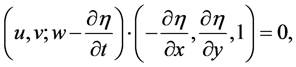
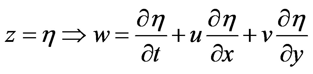 (5)
(5)
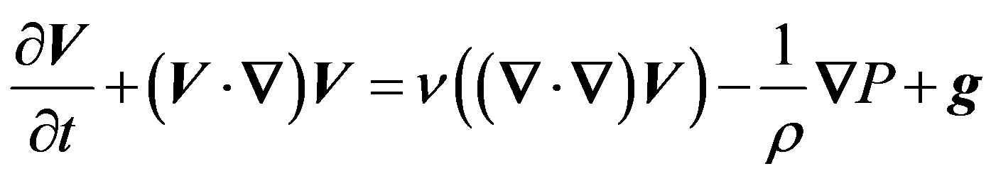
Remembering that the surface of the water is allowed to change with time. The last condition comes from the Newtonian force on a moving fluid element
 (6)
(6)
For an in viscid fluid this simplifies to
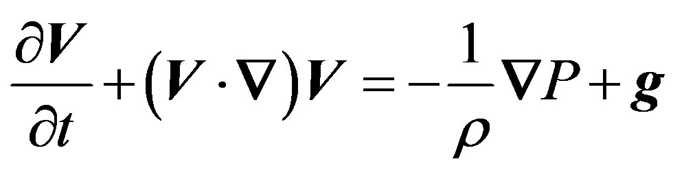 (7)
(7)
When the flow is irrotational
 (8)
(8)
We can introduce the velocity potential
 (9)
(9)
Giving the continuity equation
 (10)
(10)
The kinematic boundary condition at the bottom
 (11)
(11)
The kinematic boundary condition at the surface
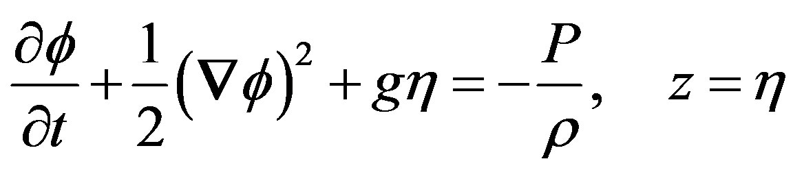
When integrating (7) with respect to x, y, z we get the Bernoulli equation, the arbitrary functions of integration ,
,  ,
,  must be the same function C(t), which can be absorbed by the velocity potential yielding exactly the same flow
Here we have made the assumption that  is constant
  making the gravitational force conservative and making it possible to define a potential energy.
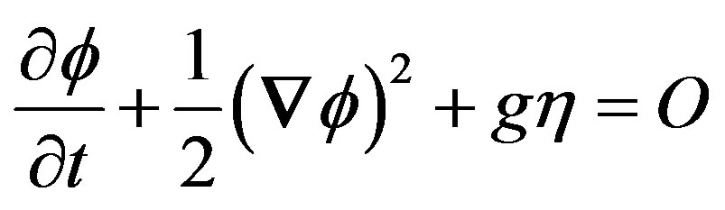
Furthermore we have made the assumption that the surface tension can be neglected. At the surface, z = h, for water flows the space above the water is the atmosphere in where the pressure is almost constant along the surface, as the density of air only about 1/800 times that of water. As this constant pressure has no important influence on the solution, we can put P = 0 giving the dynamical boundary condition at the surface of the water.
Equations (10), (11), (12), (14) are basis for all the following calculations. By introducing the stream function , defined by
 , equations (12) and (14) become:
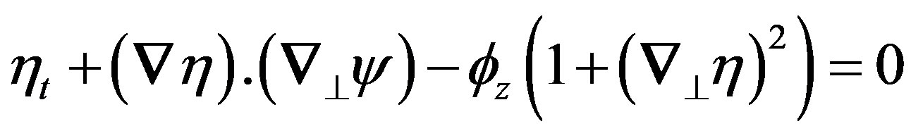 (15)
(15)
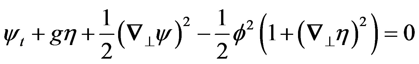 (16)
(16)
2.2. Stationary Phase Formulation of Euler Equations
The spatio-temporal evolution of the surface elevation  can be described by the reduced equation (17) of a linear wave
 (17)
(17)
The general solution of the surface elevation can be expressed as a Fourier integral
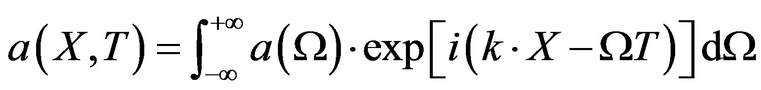 (18)
(18)
where  is obtained from (19) and
 (19)
(19)
 (20)
(20)
Boundary conditions below are used: ;
; . Fourier inverse transformation gives:
 (21)
(21)
Which solution is
Using stationary phase method [25,26], we obtain the surface elevation  expression
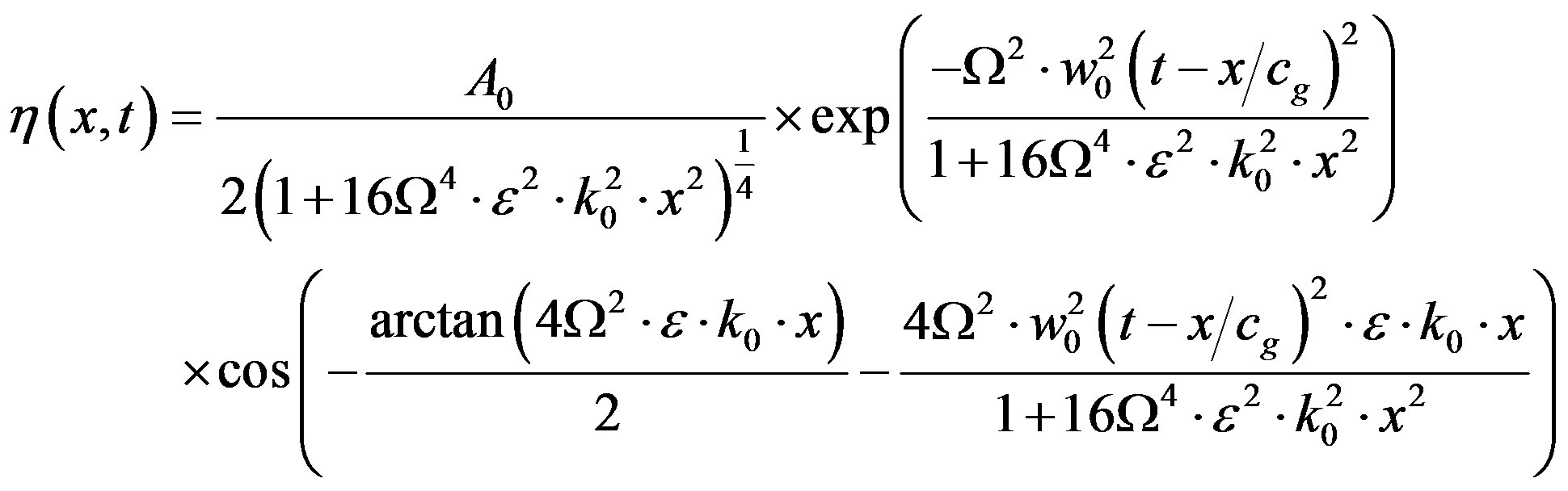
where e corresponds to the wave steepness; k0, the wave number;
 ;
; 
3. Results and Discussions
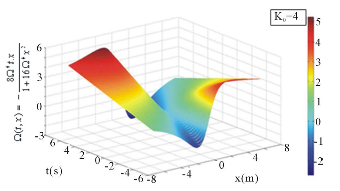
Figures presented in this manuscript provide evidence of winds stress and breaking barrier impacts on Gaussian waves. Figure 1 shows the Gaussian primary profile of the wave which is used as the target throughout the simulations. Amplitude A0 and Gaussian steepness will undergo deformations that depend on the magnitude of the wind and the proximity of the barrier (wave-barrier) located 20 m from x coordinate origin. On Figure 2(a), colors variation gives a precise idea of the impact of winds stress on the Gaussian. One can immediately notice the existence of an intense activity of wind (dark red) in the region bounded by x and t values listed in quotes {-8< x < -6; t >0}. Otherwise, the wind attacks the Gaussian basis like it was trying to move the entire structure parallel to its direction. It should however be noted that water particles located in the center of the Gaussian suffer no winds’ influence (due to the dark blue color at x = 0), the entire movement of Gaussian is then excluded and the only way allowed to the upstream side particles is to climb the Gaussian and then due to gravity fall on downstream side as illustrated on Figure 2(b). Hence the dark red color of the region bounded by {3 ˂ x˂ 8; t ˂ 0} which predicts (as t < 0) activity on the downstream side of the Gaussian.
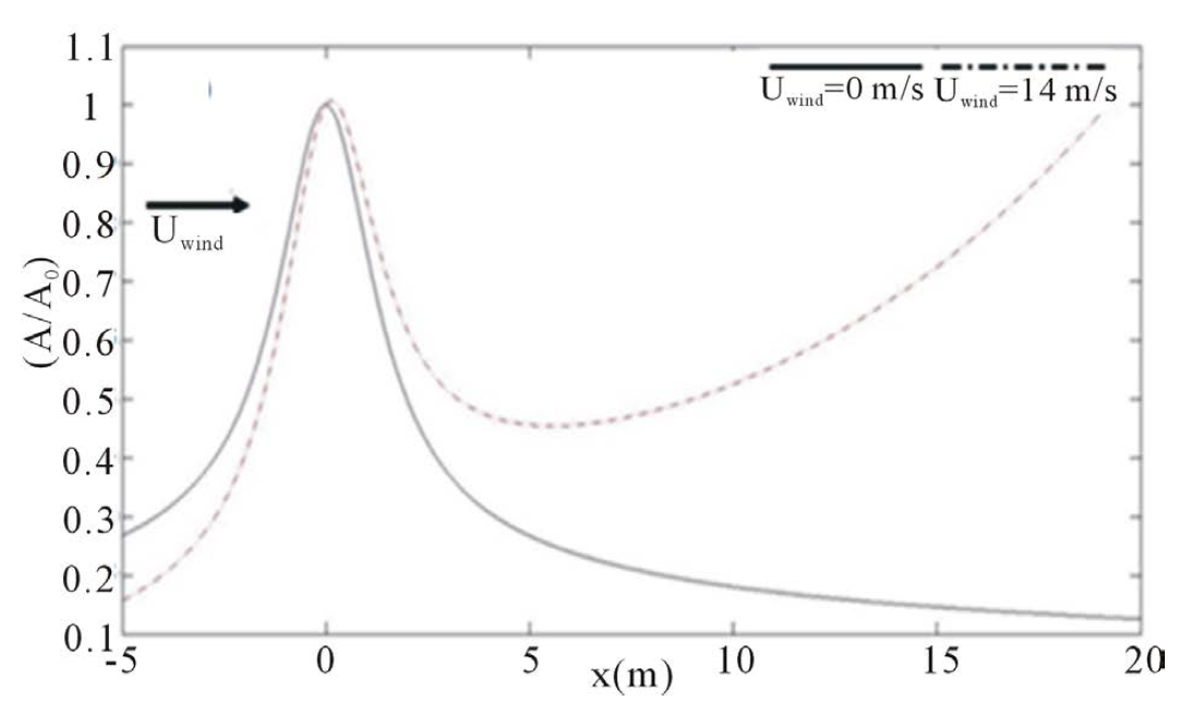
Figures 3(a)-(d) describe the Amplification Factor (A/A0) as a function of wind-magnitude. Amplification Factors are listed in Table 1. According to this table, Amplification Factor increases exponentially. All these simulations give an indication of the height to impose a barrier to prevent it being crossed by rogue waves.
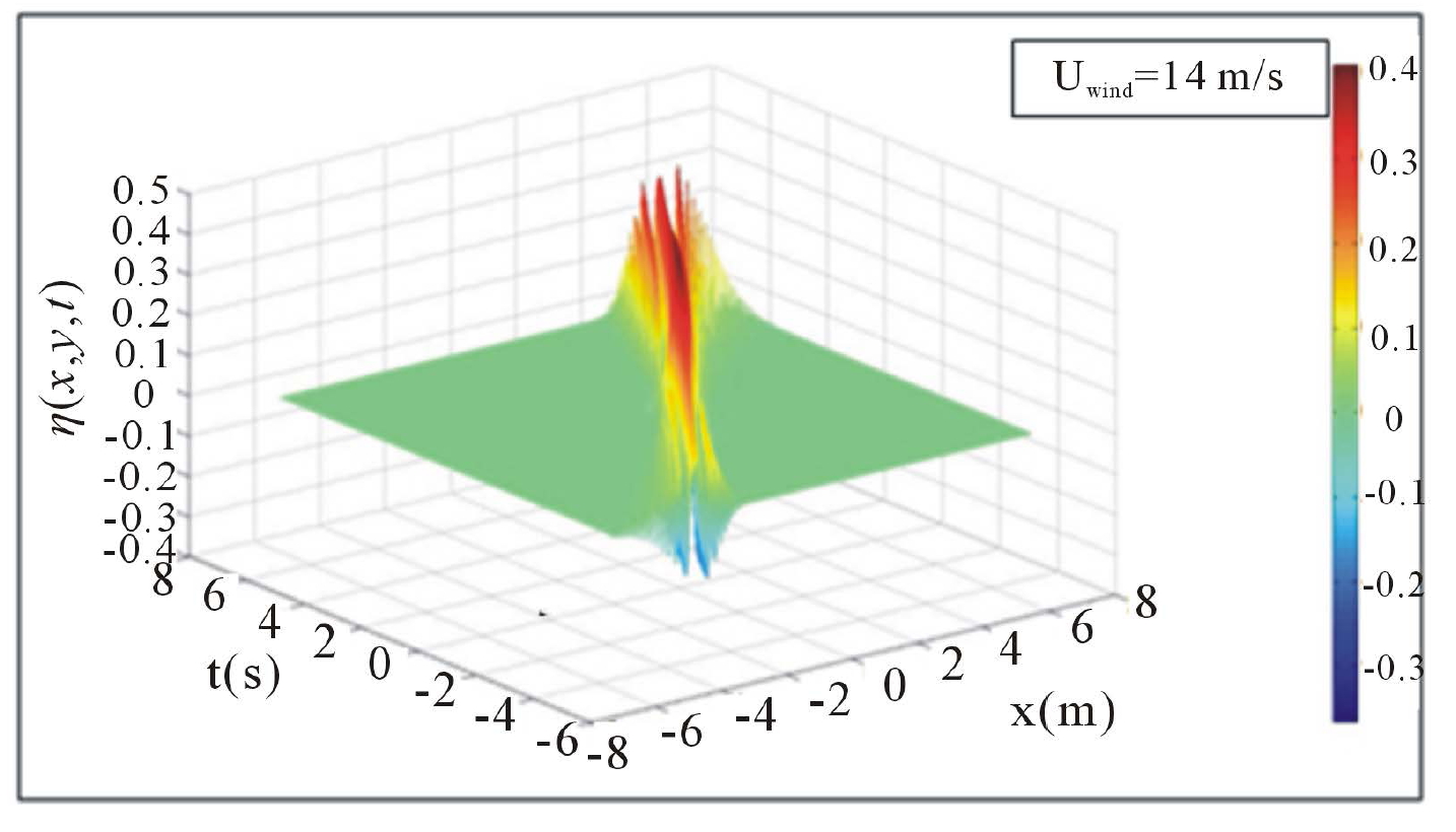
Figures 4(a)-(d), give a 3D representation of surface elevation  as a function of space and time.
One can see exactly how the target is pushed towards the barrier as the green color representing a calm ocean surface, gradually gains space when going from Figures 4(a)-(d).
4. Conclusion
Winds, as confirmed by the results obtained in this work are a serious threat to the activities on the oceans and shorelines. The wind moves the waves they meet on their way and creates relatively high waves when it causes severe depression over the oceans (e.g., tornadoes or
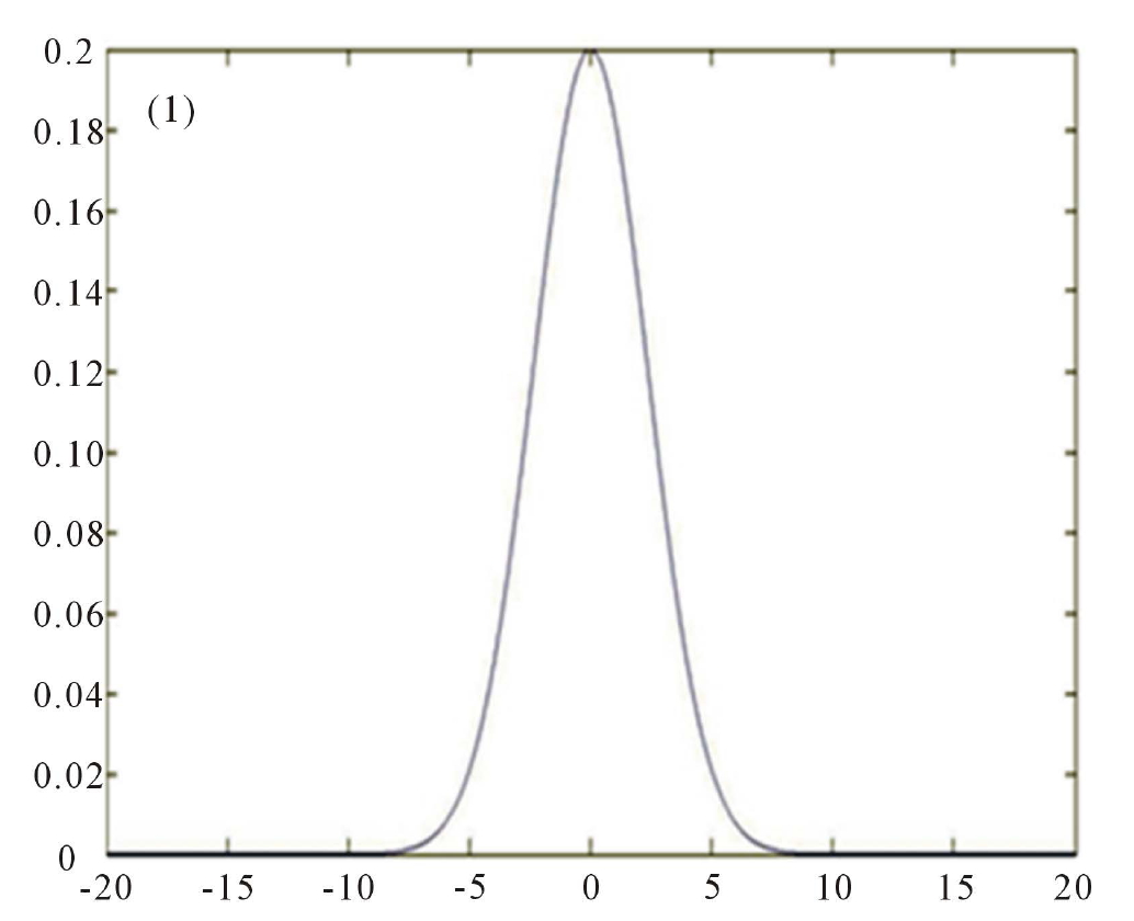
Figure 1. Profile of the primarily wave (Gaussian).
 (a)
(a)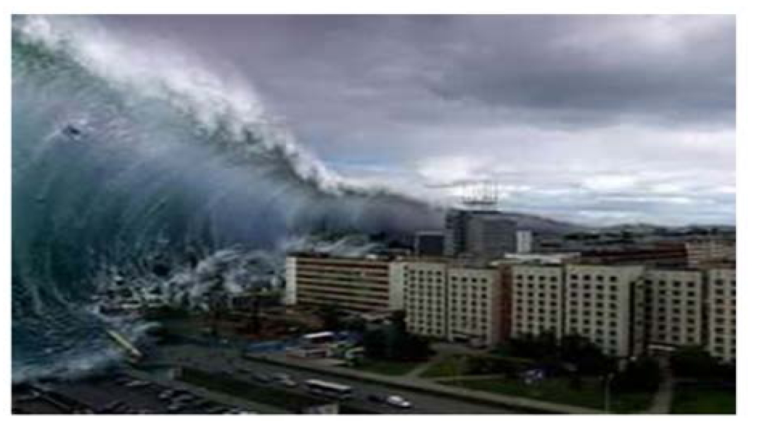 (b)
(b)
Figure 2. (a) Magnitude of winds stress impacts on the target (k0 = 4 and å = 0.4): k0 = fundamental wave number; å = small parameter of nonlinearity; (b) Rogue waves’ downstream steepness.
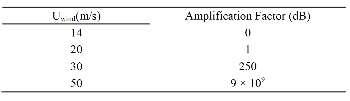
Table 1. Amplification factor as function of wind magnitude.
 (a)
(a)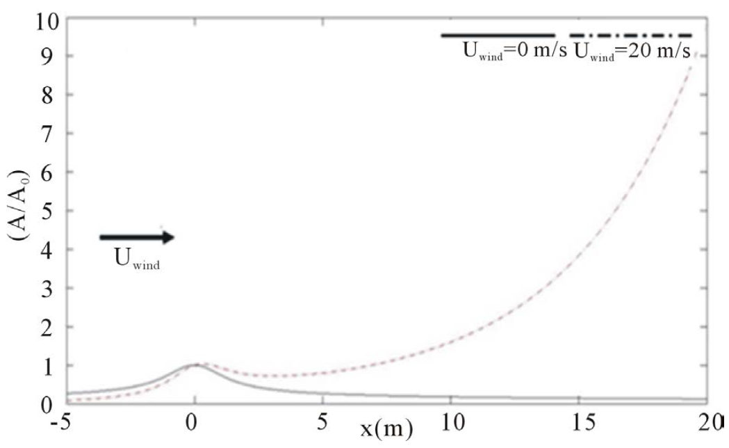 (b)
(b)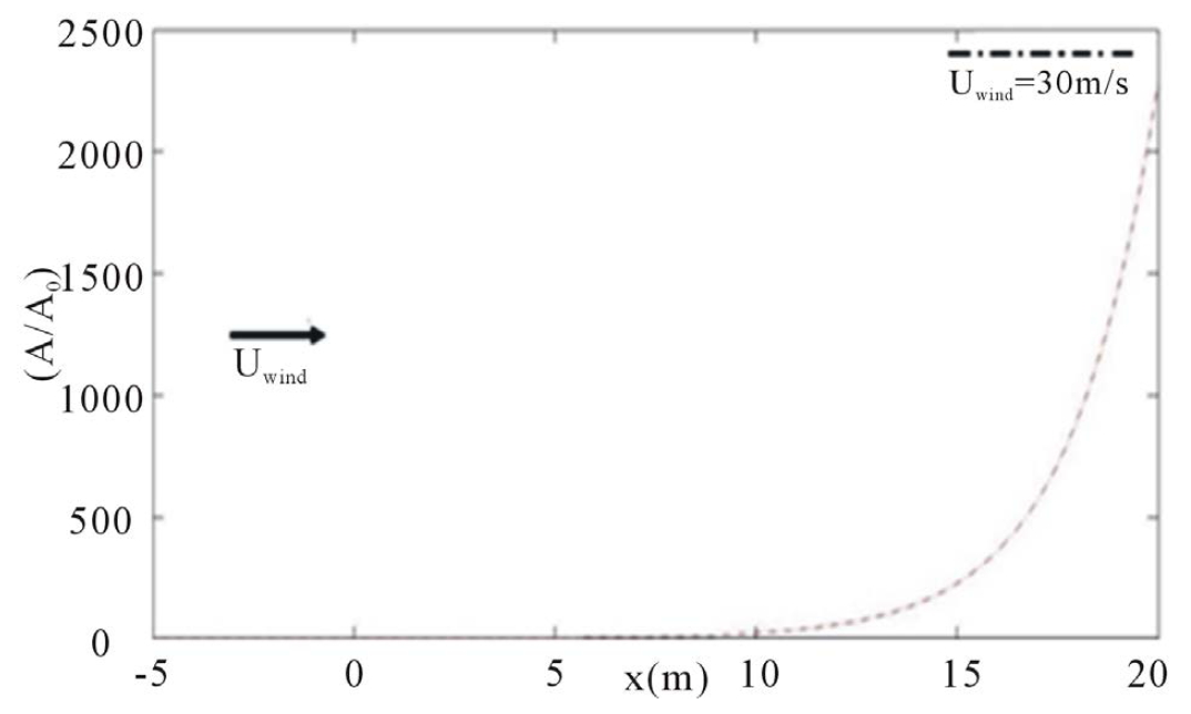 (c)
(c)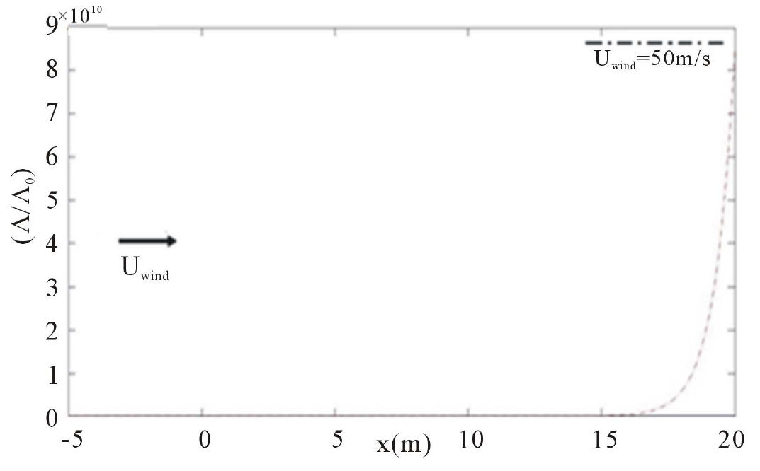 (d)
(d)
Figure 3. (a)-(d) Amplification factor for winds stress and breaking barrier impacts on a Gaussian as function of wind magnitude.
 (a)
(a)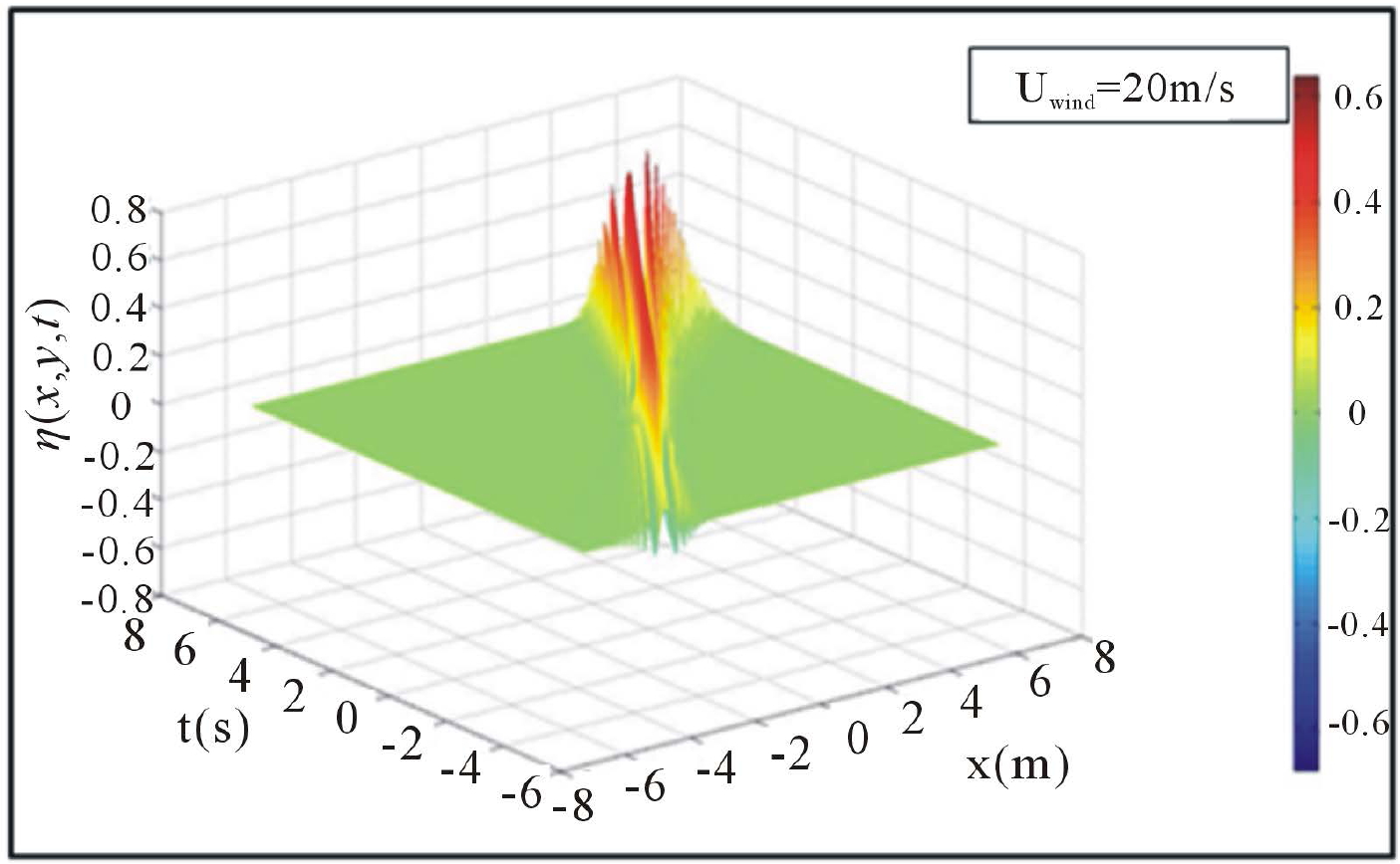 (b)
(b)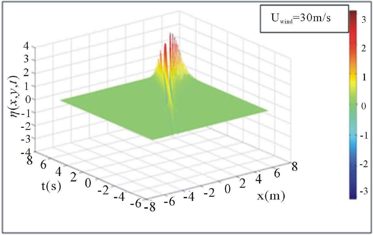 (c)
(c)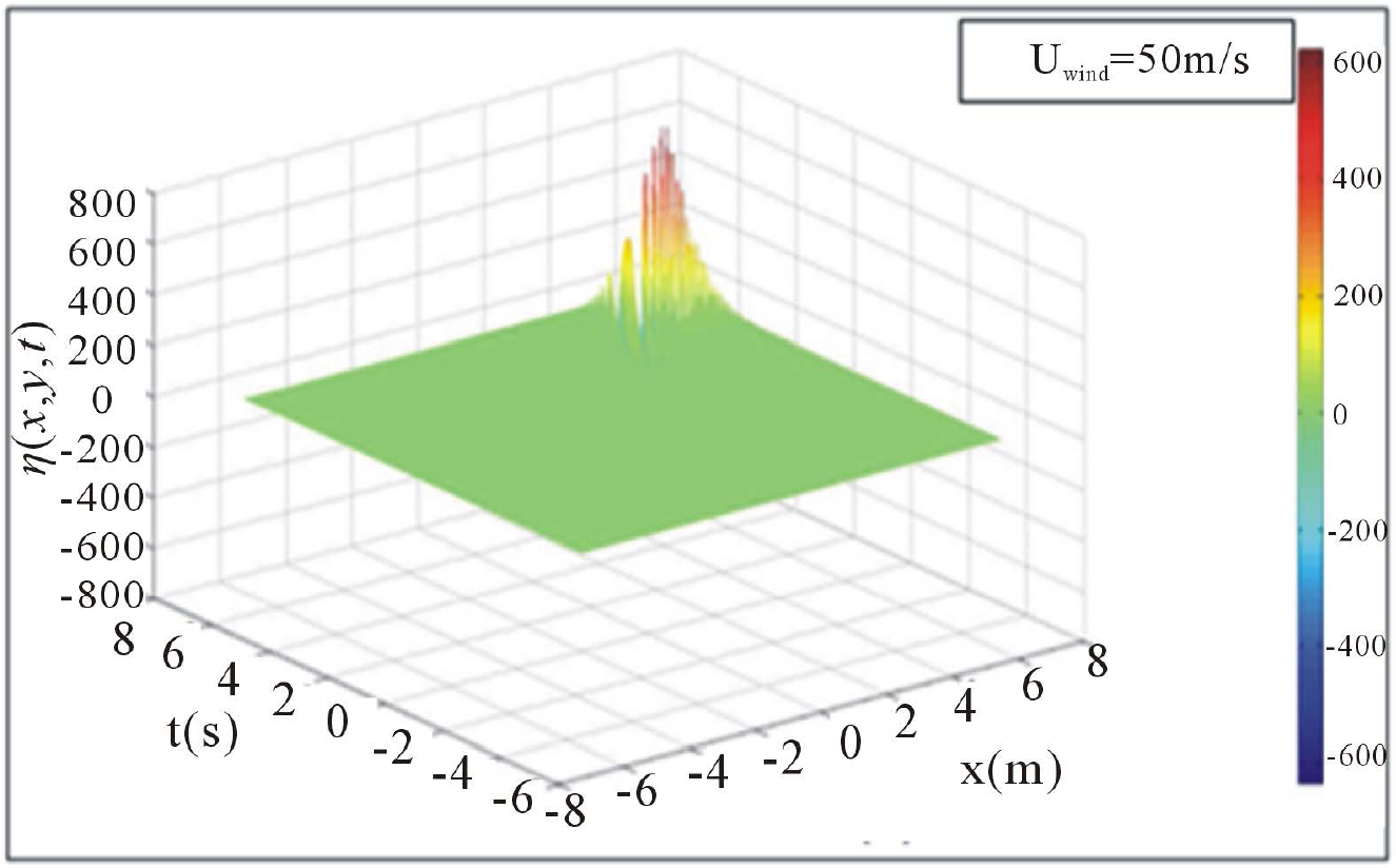 (d)
(d)
Figure 4. (a)-(d) Impacts of winds stress and breaking barrier on Surface elevation (3D-representations).
cyclones rogue waves). These results have improved our understanding of the way in which the wind acts on the granular targets and showed how difficult it is to build fences to guard against rogue waves. The choice of inputs of our model (K0 = 4, e = 0.4) is crucial for the results. But any errors can be corrected by adjusting these inputs progressively as laboratory experiments (or scientific observations) require that, if any. The oceans hostility is associated with both oceans’ impressive size that made lose all sense of direction (hence the need to embark compass and GPS) and the fear of unpredictable winds that trigger rogue waves.
REFERENCES
- J. Touboul, C. Kharif, E. Pelinovsky and J. P. Giovanangeli, “On the Interaction of Wind and Steep Gravity Wave Groups Using Miles’ and Jeffreys’ Mechanisms,” Nonlinear Processes in Geophysics, Vol. 15, 2008, pp. 1023- 1031. http://dx.doi.org/10.5194/npg-15-1023-2008
- T. B. Benjamin, “Instability of Periodic Wave Trains in Nonlinear Dispersive Systems,” Proceedings of the Royal Society of London, Vol. 299, No. 1456, 1967, pp. 59-75. http://dx.doi.org/10.1098/rspa.1967.0123
- T. Karsten and K. Igor, “On Weakly Nonlinear Modulation of Waves on Deep Water,” Physics of Fluids, Vol. 12, No. 10, 2000, pp. 24-32.
- M. Onorato, A. R. Osborne, M. Serio, L. Cavaleri and T. C. Stanberg, “Observation of Strongly Non-Gaussian Statistics for Random Sea Surface Gravity Waves in Wave Flume,” Physical Review E, Vol. 70, No. 6, 2004, Article ID: 067302. http://dx.doi.org/10.1103/PhysRevE.70.067302
- H. Socquet, A. Juglar, K. Dysthge, K. Trulsen, H. E. Krogstad and J. Liu, “Probability Distributions of Surface Waves during Spectral Change,” Journal of Fluid Mechanics, Vol. 000, 2005, pp. 1-21. http://dx.doi.org/10.1017/S0022112005006312
- A. L. Dyachenko and V. E. Zakharov, “Modulation Instability of Stokes Wave-Freak Wave,” Journal of Experimental and Theoretical Physics, Vol. 81, No. 6, 2005, pp. 318-322.
- C. Kharif and E. Pelinovsky, “Physical Mechanism of the Rogue Wave Phenomenon,” European Journal of Mechanics/B-Fluid, Vol. 22, No. 6, 2003, pp. 603-634.
- C. H. Wu and A. Yao, “Laboratory Measurements of Limiting Freak Waves on Current,” Journal of Geophysical Research, Vol. 109, 2004, pp. 1-18.
- B. S. White and B. Fomberg, “On the Chance of Freak Waves at Sea,” Journal of Fluid Mechanics, Vol. 355, 1998, pp. 113-138. http://dx.doi.org/10.1017/S0022112097007751
- C. M. Biouele, “Hurricanes and Cyclones Kinematics and Thermodynamics Based on Clausius-Clapeyron Relation Derived in 1832,” International Journal of Physical Sciences, Vol. 8, No. 23, 2013, pp. 1284-1290.
- V. E. Zakharov and N. G. Kharitonov, “Instability of Periodic Waves of Finite Amplitude on the Surface of a Deep Fluid,” Journal of Applied Mechanics and Technical Physics, Vol. 11, 1970, pp. 747-751.
- L. Shener, “On Benjamin-Feir Instability and Evolution of Nonlinear Wave with Finite-Amplitude Side Bands,” Natural Hazards and Earth System Sciences, Vol. 10, 2010, pp. 2421-2427. http://dx.doi.org/10.5194/nhess-10-2421-2010
- S. Leblanc, “Wind-Forced Modulations of Finite—Dephgravity Waves,” Physics of Fluids, Vol. 20, No. 11, 2008, Article ID: 116603. http://dx.doi.org/10.1063/1.3026551
- K. Batra, R. P. Sharma and A. D. Verga, “Stability Analysis on Nonlinear Evolution Paterns of Modulational Zakharov Equations,” Journal of Plasma Physics, Vol. 72, No. 5, 2006, pp. 671-686. http://dx.doi.org/10.1017/S002237780500423X
- M. I. Banner and J. B. Song, “On Determining the Onset and Strength of Breaking for Deep Water Waves. Part ii: Influence of Wind Forcing and Surface Shear,” Journal of Physical Oceanography, Vol. 32, No. 9, 2002, pp. 2559- 2570. http://dx.doi.org/10.1175/1520-0485-32.9.2559
- M. G. Brown and A. Jensen, “Experiments on Focusing Unidirectional Water Waves,” Journal of Geophysical Research, Vol. 106, No. C8, 2001, pp. 16917-16928. http://dx.doi.org/10.1029/2000JC000584
- H. Jeffreys, “On the Formation of Wave by Wind,” Proceedings of the Royal Society A, Vol. 107, No. 742, 1925, pp. 189-206. http://dx.doi.org/10.1098/rspa.1925.0015
- O. M. Philips, “On the Interaction of Waves by Turbulent Wind,” Journal of Fluid Mechanics, Vol. 2 1957, pp. 417- 455.
- V. K. Makin, H. Branger, W. L. Peirson and J. P. Giovanangeli, “Stress above Wind-plus-Paddle Waves: Modeling of a Laboratory Experiment,” Journal of Physical Oceanography, Vol. 37, No. 12, 2007, pp. 2824-2837. http://dx.doi.org/10.1175/2007JPO3550.1
- J. W. Miles, “On the Generation of Surface Wave by Shear Flow,” Journal of Fluid Mechanics, Vol. 3, No. 2, 1957, pp. 185-204. http://dx.doi.org/10.1017/S0022112057000567
- L. Shemer, K. Goulitski and E. Kit, “Evolution of Wide Spectrum Unidirectional Wave Groups in a Tank: An Experimental and Numerical Study,” European Journal of Mechanics—B/Fluids, Vol. 26, No. 2, 2007, pp. 193- 219. http://dx.doi.org/10.1016/j.euromechflu.2006.06.004
- J. B. Song and M. I. Banner, “On Determining the Onset and Strength of Breaking for Deep Water Waves, Part i: Unforced Irrotational Wave Groups,” Journal of Physical Oceanography, Vol. 32, No. 9, pp. 2541-2558. http://dx.doi.org/10.1175/1520-0485-32.9.2541
- T. Stanton, D. Marshall and R. Houghton, “The Growth of Waves on Water Due to the Action of the Wind,” Proceedings of the Royal Society A, Vol. 137, No. 832, 1932, pp. 283-293. http://dx.doi.org/10.1098/rspa.1932.0136
- A. Daika, H. M. Etoundi, C. M. Ngabireng and C. Mbané- Biouélé, “Application of Benjamin-Feir Equations to Tornadoes’ Rogue Waves Modulational Instability Inoceans,” International Journal of Physical Sciences, Vol. 7, No. 46, 2012, pp. 6053-6061.
- M. Talon, “Ondes de Surface,” LIPTHE Paris VI-CNRS, 2006.
- J. W. Miles, “Surface-Wave Generation: A Viscoelastic Model,” Journal of Fluid Mechanics, Vol. 322, 1996, pp. 131-145. http://dx.doi.org/10.1017/S002211209600273X
List of Symbols
Physical Symbols
b: Complex surface function Bi: Main component of the complex surface function (i = 0,1,2,3)
 : Smaller component of the complex surface function (i = 0,1,2,3)
 : Smallest component of the complex surface function (i = 0,1,2,3)
g: Acceleration of gravity
 : Three-dimensional acceleration of gravity H: Water depth ki: Wave number (i = 0,1,2,3)
 : Wave number vector (i = 0,1,2,3)
P: Pressure t: fast time scale t1: Slower time scale t2: Slowest time scale Vi: Interaction coefficient (i = 0,1,2,3)
w: Vertical velocity of particle Wi: Interaction coefficient b(ki) = bi: Main component of the complex surface function (i = 0,1,2,3)
e: Measure of non-linearity’s (steepness)
f: Velocity potential h: Surface elevation ht: Derivative of the surface elevation h with respect to time y: Stream function yt: Derivative of the stream function y with respect to time w(ki) = wi: Angular frequencies of interaction waves
Mathematical Symbols
d: Dirac’s d-function
 : Three-dimensional gradient
 : Vertical component of the gradient
*: complex conjugate
Dispersion Coefficients
Cx,y = Group velocity components t, V, J = Group dispersion coefficients x = Non-linear coefficient z = Coupling coefficient
NOTES
*Corresponding author.