Open Journal of Ecology
Vol.2 No.2(2012), Article ID:19500,4 pages DOI:10.4236/oje.2012.22008
Landscape spatial structure for predicting suitable habitat: The case of Dalea villosa in Saskatchewan
![]()
1Department of Geography and Planning, University of Saskatchewan, Saskatoon, Canada; *Corresponding Author: shl314@mail.usask.ca
2Environmental Stewardship Branch, Prairie and Northern Canadian Wildlife Service, Environment Canada, Saskatoon, Canada
Received 28 February 2012; revised 2 April 2012; accepted 18 April 2012
Keywords: Spatial Structure; Habitat Pattern; Remote Sensing; Habitat Suitability; Rare Plants
ABSTRACT
Prediction of potentially suitable habitat is important for the recovery of species protected by federal laws. Therefore, the objective of this research was to study the relationship between habitat configuration and hairy prairie-clover occurrence in order to predict suitable and unsuitable bare sand habitat across the study site. Bare sand patches were extracted from a land cover classification of the study site and several patch scaled metrics were calculated to characterize habitat spatial structure. Binary logistic regression was used to determine which metrics were significantly correlated with hairy prairie-clover occurrences. The logistic regression equation was subsequently used to predict suitable and unsuitable bare sand habitat for hairy prairie-clover based on the probability of occupancy. Results showed that about 29% of the variation in bare sand patch occupancy could be explained by the size, shape, and degree of isolation of a sand patch as well as the amount of vegetation on a sand patch in the early growing season. Based on these variables, 18.8% of bare sand patches in the study site were predicted to be unsuitable hairy prairieclover habitat, 45.7% were predicted to be marginally unsuitable, 32.7% were predicted to be suitable, and 2.8% were predicted to be marginally suitable.
1. INTRODUCTION
One challenge with predictive modelling is that many species records include presence-only data with no reliable records of absences. Popular methods such as GARP (Genetic Algorithm for Rule-set Prediction), BioClim, and Maxent have proven accuracy for modelling when presence-only data is available for a species [1,2]. However, evaluating model performance for presence-only methods still requires the use of presence/absence data. Evaluating model performance with presence-only data limits the options for the data set and the power of statistical evaluations [1]. Therefore, where reliable presence/absence data sets are available, it is best to choose methods such as generalized linear models, generalized additive models, regression-based models, or resource selection functions [2,3]. Further, most theoretical models assume that response curves are either sigmoid or guassian, although in real ecological systems guassian curves may be rare due to factors such as thresholds along an environmental gradient or interspecific interactions. Therefore, regression-based habitat suitability models, such as logistic regressions, may be a better choice because they can fit curves ranging from parametric functions to less constrained shapes [3].
For plant species occupying discrete habitat niches, such as in the case of hairy prairie-clover, habitat suitability modeling can be effectively applied [4]. The ecological niche concept is based on the theory that species only thrive in discrete ranges of environmental conditions [3]. However, due to abiotic and biotic interactions with the surrounding environment a species may be constrained to occupy only a subset of its fundamental niche. This subset can be described as the realized niche. Habitat suitability modeling is an application of the ecological niche theory because it aims to predict the probability of occurrence of a species based on environmental conditions. The geographical distribution of a species generally follows three constraints: 1) the local environment allows the population to grow, 2) interactions with other local species allow the species to persist, and 3) the location is accessible given the dispersal abilities of the species [3]. Therefore, habitat suitability modeling can only reconstruct the realized niche for a species based on the environmental variables present in the locations it occupies [5].
When dealing with plant species, it is important to consider that they are immobile, exhibit a strong spatial structure through specific habitat preferences, and their dispersal is restricted [4]. Therefore, the geographical distribution of a plant species is heavily dependent on the geographical distribution of its realized niche. Thus, the above three constraints can be equated to functions of patch area, patch quality, and patch isolation, respectively [6]. The three most basic processes determining the survival of a local population patch are dispersal, establishment, and persistence [4]. It has been adequately documented that dispersal is mainly affected by patch isolation and matrix quality; establishment depends on patch size, number of patches, and patch quality; and persistence depends on patch size and patch quality [7,8]. Sensitivity to these spatial factors has been noted to be higher in rare species and habitat specialists as opposed to generalist species because they tend to have lower reproductive outputs, have shorter lived seeds, are smaller in size, and are geographically restricted [8,9].
Many habitat suitability models still fail to be successfully applied to real ecological problems because they fail to address spatial structure through assuming that all patches are equivalent in size and quality, and that all local populations are equally accessible by dispersers. Considering that all plant populations are spatially structured, habitat pattern must be incorporated into habitat suitability models to allow for an ecologically meaningful interpretation [10]. However, a distinction between habitat parameters that can be mapped and measured versus habitat parameters that are ecologically relevant must be made [11].
For hairy prairie-clover, the dominant habitat requirement appears to be an element of bare sand cover resulting in the plants confinement to geographical features such as parabolic sand dunes, stabilized blow-outs, dune depressions, and sand flats [12]. It has been identified that factors such as climate change, vegetation encroachment, invasive species encroachment, anthropogenic sources and land use changes, and loss of natural disturbance by bison and fire have contributed to the reduction in sand dune activity and bare sand areas within the prairies [13-15]. The association of hairy prairie-clover with these types of bare sand areas makes it particularly vulnerable to changes in habitat pattern as incurred by the above factors. It has also been identified that vegetation and invasive species encroachment of bare sand and sand dune areas, loss of grazing and fire disturbance pressures, and changes in land use patterns are the main threats to the survival of hairy prairie-clover [12]. Thus, it is hypothesised that the dominant factor limiting the abundance of hairy prairie-clover on the landscape is the spatial configuration of bare sand areas in context to other landscape elements.
The purpose of this research was to analyse habitat pattern to gain an understanding of the spatial structure of bare sand habitat for hairy prairie-clover and to predict potentially suitable and unsuitable habitat for this plant. There were two specific research questions: 1) What is the spatial pattern of intra-patch and inter-patch characteristics for occupied and unoccupied bare sand habitat? and 2) What spatial configuration of bare sand habitat best explains and predicts occupancy by hairy prairie-clover?
2. METHODS
2.1. Study Site
This study took place in south central Saskatchewan within the Dundurn and Rudy Rosedale Prairie Farm Rehabilitation Administration (PFRA) Community Pastures located at 51˚45’00”N and 106˚45’00”W (Figure 1). The area is a remnant patch of natural mixed-grass prairie and sand dune complexes bordered on the north
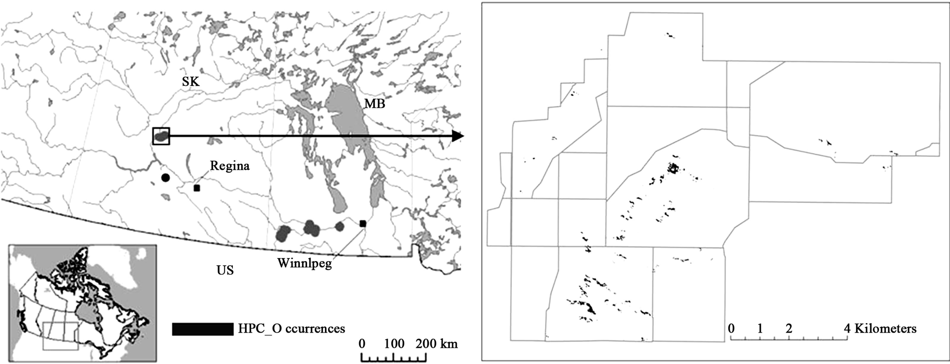
Figure 1. Dundurn and Rudy Rosedale Prairie Farm Rehabilitation Administration Community Pastures, Saskatchewan. The Canadian distribution of hairy prairie-clover (HPC) is shown on the left [20]. A close-up of the study site is shown on the right with pasture boundaries outlined in grey. The known distribution of the population is shown by the black polygons.
by the Canadian Forces Base, 17-Wing Detachment Dundurn, the east and south by mixed farm land, and the west by highway #219. The landscape is dominated by five main land cover types; aspen (Populus tremuloides Michx.), shrub (Elaeagnus commutata Bernh. ex. Rydb., Prunus virginiana L. var. virginiana, Symphoricarpos occidentalis Hook.), juniper (Juniperus horizontalis Moench.), grassland, and sand dunes. This pasture is categorized as a low dunes ecosite with mainly stabilized sandy hills that have gentle to moderate slopes and areas between dunes that are relatively flat comprising a mixed-grass community [16].
The sand dunes found in the Dundurn area comprise four physiographic categories: active complexes, stabilized blow-outs, stabilized dunes, and dune depressions. Species most commonly associated with active complexes are Psoralea lanceolota, Agropyron spp., and Lygodesmia juncea. Stabilized blow-outs are saucer-shaped depressions oriented in the direction of the prevailing wind and are most often vegetated by Juniperus horizontalis, Carex heliophila and Selaginella densa. When dunes become stabilized, the resulting vegetation community is most dominated by Stipa comata, Artemisia frigida, and Selaginella densa. The difference between stabilized blow-outs and stabilized dunes is seen in the occurrence of low lying shrubs on the former which are less common on stabilized dunes. The dominant species in dune depressions, which occur on stabilized dunes, are Stipa comata, Calamovilfa longifolia and Agropyron spp. [17]. Many population patches of hairy prairie-clover have been found in grassland and prostrate shrub stands within the study site, most commonly on low angled south and west facing slopes with partial vegetation cover and exposed sand [18].
This PFRA pasture covers an area of 1.23 108 m2 with a maximum altitude of 520 m. The Dundurn sand hills are characterized by annual temperature extremes with a mean annual temperature of 2.2˚C and a mean of 14.8˚C during the growing season from May to September [19]. The growing season is short with about 105 frost free days, high wind speeds (mean annual wind speed of 15.7 km hr–1), high evaporation rates (mean annual evaporation rate of 650 mm), and low precipitation rates (mean annual precipitation rate of 350 mm) [19]. Prevailing winds in southern Saskatchewan are from the northwest resulting in a general dune orientation of northwest to southeast.
2.2. Data Set
2.2.1. Land Cover Classification
A SPOT5 panchromatic image (wavelengths 490 - 690 nm) at 2.5 m spatial resolution was acquired on April 13, 2007. This imagery was selected for its high spatial resolution. Three SPOT5 multispectral images (green, red, Near Infra-Red (NIR), and Mid Infra-Red (MIR) bands) at 10 m spatial resolution were acquired on May 27, 2009; July 12, 2009; and August 16, 2007. These images were selected for the multiple bands and covering three stages of the growing season.
A multi-temporal, multi-resolution land cover classification was carried out using object-oriented methods. Class boundary delineation was completed using a multiresolution segmentation algorithm at a scale parameter of ten, with shape and compactness weighted at 0.1 and 0.5 respectively. Following segmentation, the landscape was classified in to the five main land cover types present in the study site: aspen, shrub, juniper, grassland, and bare sand with a sixth class, other, added during post classification editing. A nearest neighbour classifier was set up using twenty six training data points collected in the field for each class and class membership values were assigned based on the mean reflectance within the panchromatic, red, NIR, and MIR bands of an object. A hierarchical rule set was developed to maximize spectral and shape separability between classes.
The raster data format of the land cover classification was converted to vector data, retaining the original boundaries of raster data. Bare sand patches were extracted from the classification and dissolved to create a separate layer of the class bare sand. The remote sensing data set consisted of the bare sand layer.
2.2.2. Occupancy Data for Hairy Prairie-Clover
Occupancy data for hairy prairie-clover was collected between 2007 and 2010. A previous coarse resolution land cover map from Environment Canada was used to identify 351 patches within which to restrict groundbased searches for hairy prairie-clover. Systematic searches of these patches were conducted from July to September each year to allow for easy detection as the plant is in bloom during this time period. Searches included a complete search of the bare sand patch and a buffer area of 30 m surrounding each patch. If plants were found, the outer boundary of the population was tracked using GPS (+/– 5 m error) to record the spatial extent of the patch. In spatial analyses, pseudo replication of a variable will depend on the distance between the sample points, such that a set of closely spaced sample points will be spatially autocorrelated and thus decrease the effective sample size [2]. Therefore, to minimize spatial autocorrelation issues, any hairy prairie-clover plants that were found within a 30 m proximity of one another were counted as the same patch/population.
This polygonal occupancy data was overlayed on the bare sand layer extracted from the above land cover classification to create an attribute table for bare sand patches where hairy prairie-clover was present or absent. Presence/absence data from 2007-2009 was used as training data in model building while presence/absence data collected in 2010 was kept separate for use as validation data in accuracy assessment. Reference [21] found that regular and equal-stratified sampling designs were the most accurate and robust for habitat suitability and presence/absence predictions. However, gradients that exert major control over a species distribution should be used to stratify sampling and increase efficiency [21]. Therefore, in this case it was most appropriate to use systematic searches of targeted bare sand areas in data collection.
2.3. Metrics for Bare Sand Patch Configuration
To determine inter and intra patch spatial characteristics of bare sand patches, patch scaled metrics were calculated. Metrics were chosen based on the premise that the likelihood of a species occupying a particular habitat niche is a function of patch area and patch isolation [6]. In plant species, dispersal can be affected by patch isolation, establishment by the availability of suitable habitat and habitat quality, and persistence by patch size [8]. Therefore, six metrics were calculated for bare sand patches: area, shape, fractal dimension, Euclidean nearest neighbour distance, proximity count, and proximity percent. The normalized difference vegetation index (NDVI) was also calculated as a measure of habitat quality.
Shape was calculated as
 (1)
(1)
where pij is the patch perimeter and aij is the patch area, adjusted by the constant 0.25 to adjust for the square standard in raster data [22]. Shape will equal one if a patch is perfectly square and increase without limit as patch shape becomes more irregular [22]. It is a unitless measure. Fractal dimension, another measure of patch shape, was calculated as
 (2)
(2)
where pij is the patch perimeter, aij is the patch area, 0.25 is the constant for the square standard in raster data, and ln is the natural logarithm [22]. Fractal dimension will vary between a value of one and two (unitless), where one signifies a square patch and two is the upper limit of shape irregularity [22].
The Euclidean nearest neighbour (ENN) distance was calculated as the straight line distance (meters) between the centroids of the closest neighbouring patches. Bare sand patch centroids were created based on the gravimetric center of patches. Proximity measures, as a representation of patch isolation, were based on a 30 m buffer zone surrounding bare sand patches. Proximity count is the number of bare sand patches that fall within the 30 m buffer zone of the target sand patch. Proximity percent is the percentage of the area of the 30 m buffer zone that is of the bare sand class. These measures were modified from the proximity index by [22] to create a more meaningful output. Given that hairy prairie-clover spreads mainly by seed [18], it is plausible that dispersal distances fall within this proximity.
In plant species, one aspect of habitat quality is the competition for resources with other flora species, especially in inferior competitors because plants are immobile [3]. Therefore, it is important to consider the amount of vegetation growing on bare sand patches as one measure of habitat quality for hairy prairie-clover. NDVI was used as a surrogate measure of the amount of vegetation on a bare sand patch. NDVI can be calculated for an image on a per-pixel base as
 (3)
(3)
The difference in reflectance between the red band (absorption in vegetation, reflectance in soil) and NIR band (reflectance in vegetation and soil) will enhance vegetation signal across the imagery. NDVI is one of the most popular vegetation indices because it can capture seasonal changes in vegetation growth, it is highly correlated with leaf area index, and it works best in low biomass conditions such as grassland, semi-arid, and arid regions [23]. NDVI was calculated for the SPOT5 multispectral images from August and May. NDVI from August was chosen because during the late growing season, the maximum amount of vegetation coverage on a bare sand patch will show up [23]. NDVI from May was also chosen to show the amount of vegetation on a bare sand patch in the early growing season. Competition for resources in the early growing season can affect seedling establishment and persistence which is important for population growth [3,24]. The average NDVI for each sand patch was calculated.
2.4. Statistical Analysis and Model Building
Bare sand patches were coded based on hairy prairieclover occupancy data where zero was unoccupied, one was occupied, and two was unknown. The data set consisted of 314 occupied and 314 unoccupied bare sand patches randomly selected from the 2007-2009 occurrence data. Using a binary response variable in logistic regression is a popular approach to habitat suitability modelling [21]. However, sampling of the data should be done in a way to reduce model bias. Therefore, equal sample sizes were chosen to represent occupied and unoccupied sand patches. The independent variables tested were area, shape, fractal dimension, Euclidean nearest neighbour distance, proximity count, proximity percent, mean NDVI August, and mean NDVI May. For all tests, α = 0.05 was used. Assumptions of normality were tested using the one-sample Kolmogorov-Smirnov test. For independent variables in normal distribution, the independent-samples t-test was used to test for a significant difference between occupied and unoccupied bare sand patches. Assumptions of equal variances were tested using Levene’s test for equality of variances. The independent-samples Mann-Whitney U test was used to test for a significant difference between occupied and unoccupied bare sand patches for variables not in normal distribution [25].
Binary logistic regression was used to determine which independent variables were significantly correlated with hairy prairie-clover occurrences, because the dependent variable was binary and the independent variables were continuous [25]. Logistic regression is advantageous because it provides an equation for predicting the probability of occupancy on a bare sand patch, it uses multivariate comparisons between occupied and unoccupied sand patches, and it can identify the variables most associated with the occurrence of hairy prairie-clover [26]. The stepwise selection of independent variables can be useful for selecting an optimal model because the full model may be oversized, overfitted, or redundant [2]. Therefore, a forward stepwise likelihood ratio method was used (enter 0.05, removal 0.10). Correlation between independent variables can influence the final model because the selection and contribution of a variable depends on other variables already in the model [26]. Therefore, to avoid multicollinearity, only shape was used in the logistic regression and not fractal dimension. Mean NDVI August was also left out of the model because there was no significant difference between occupied and unoccupied bare sand patches for this variable (P > 0.05). Variables considered in the model were area, shape, Euclidean nearest neighbour distance, proximity count, proximity percent, mean NDVI May, and all possible interactions. The Hosmer-Lemeshow test was used to test the assumption that there is a linear relationship between the independent variables and the log odds of the dependent variable [25].
2.5. Habitat Suitability Predictions and Model Validation
The logistic regression equation was subsequently used to calculate the probability of occupancy for all bare sand patches. Probability of occupancy was calculated as
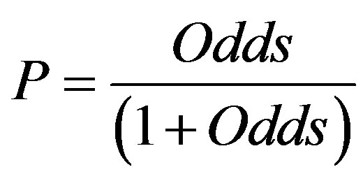 (4)
(4)
where odds was defined as
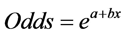 (5)
(5)
with a + bx being the logistic regression equation. Hairy prairie-clover occupancy data from 2010 was used for accuracy assessment of model predictions. The data set consisted of 377 unoccupied and 131 occupied sand patches. Hairy prairie-clover occurrence polygons were overlaid with the bare sand layer to create a contingency table of the model predictions (predicted suitable/unsuitable) against actual observations (observed presence/ absence) (Table 1).
The Kmax index is the highest kappa value achieved when calculating the kappa coefficient at all threshold values between zero and one [1,27]. It is a threshold-independent evaluator. Contingency tables were constructed for threshold values 0.1, 0.2, 0.3, 0.4, 0.5, 0.6, 0.7, 0.8, and 0.9. Threshold values are defined in Table 2. The kappa coefficient was calculated for each threshold value as
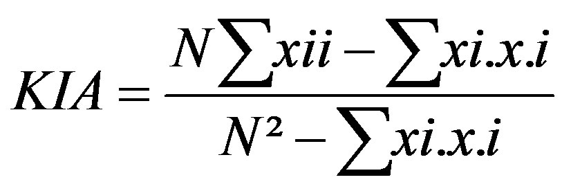 (6)
(6)
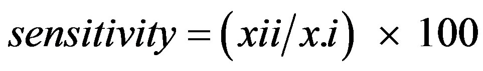
where x and N are counts of evaluation points as defined in Table 1 [27]. The percentage of presences correctly predicted was calculated from the contingency tables as
 (7)
(7)
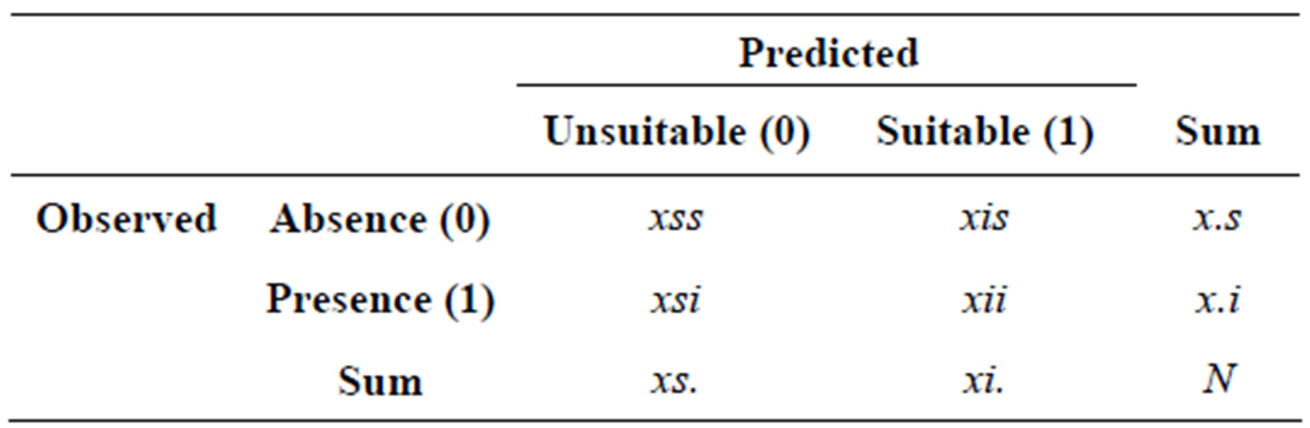
Table 1. Contingency table for calculation of KIA, sensitivity, specificity, and overall %.
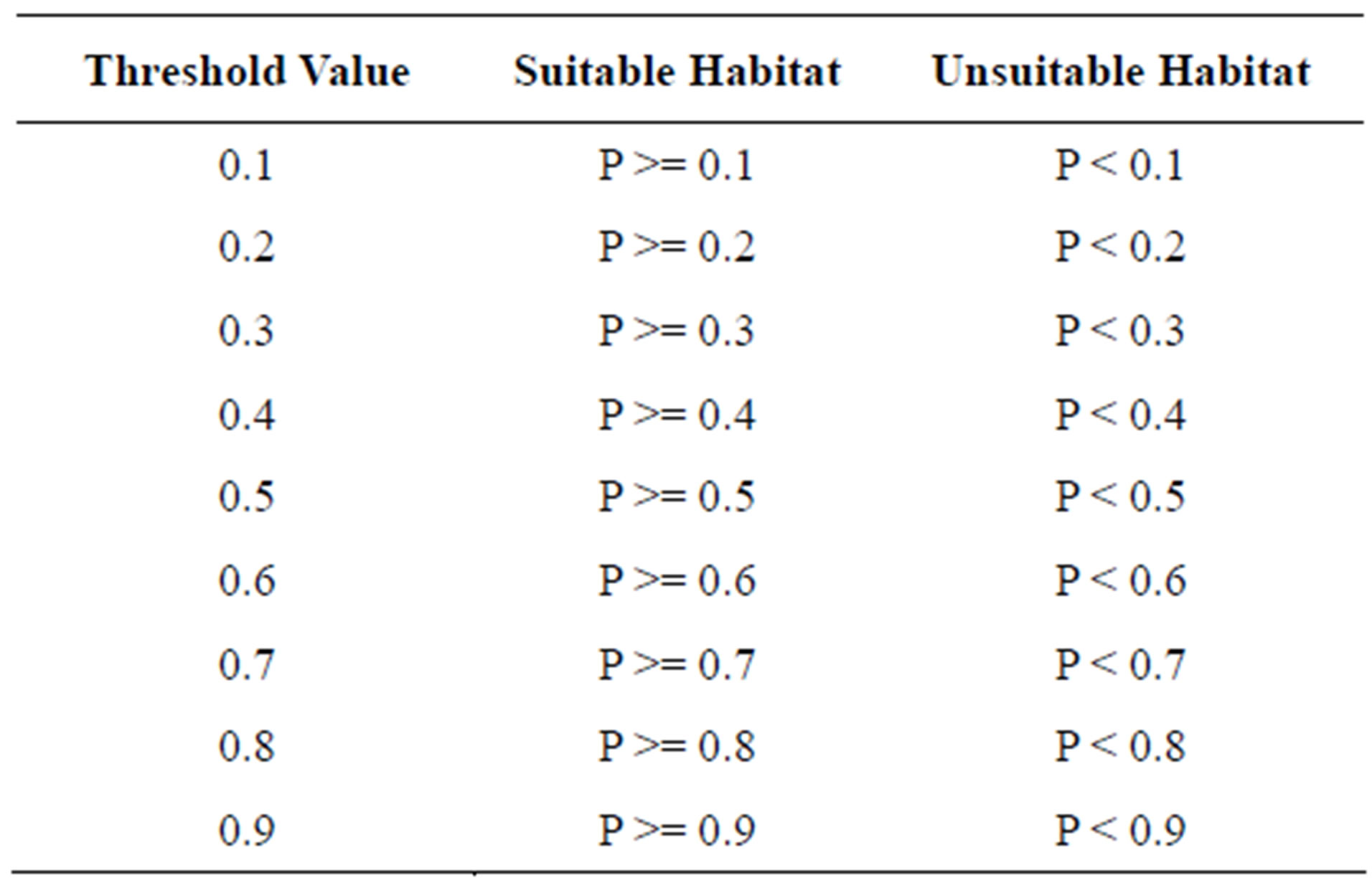
Table 2. Predicted suitable and unsuitable hairy prairie-clover habitat based on probability of occupancy for threshold values varying between zero and one. P represents the probability of occupancy for a bare sand patch and varies between zero and one.
where xii and x.i are defined in Table 1. The percentage of absences correctly predicted was calculated from the contingency tables as
 (8)
(8)
where xss and x.s are defined in Table 1. The overall percentage correctly predicted was calculated from the contingency tables as
 (9)
(9)
where N is defined in Table 1.
The area under curve (AUC) is one of the most common threshold-independent methods for evaluating species’ distribution models because it allows one to weight the risks of over and under predicting species’ presences [1,27]. For each threshold value the true-positive ratio was plotted against the false-positive ratio and the area under the resulting curve was calculated. As well, a second curve was plotted with the true-negative ratio against the false-negative ratio for calculation of the area under the curve. The true-positive ratio was calculated from the contingency tables as
 (10)
(10)
as defined in Table 1 [27]. The false-positive ratio was calculated from the contingency tables as
 (11)
(11)
as defined in Table 1 [27]. The true-negative ratio was calculated from the contingency tables as
 (12)
(12)
as defined in Table 1 [27]. The false-negative ratio was calculated from the contingency tables as
 (13)
(13)
as defined in Table 1 [27]. The AUC value will vary between zero (worse than random model) and one (best possible model), with values of 0.70 and greater indicating average to excellent model accuracy [2].
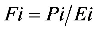
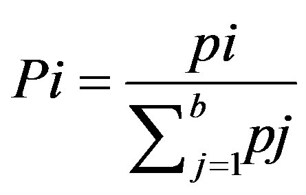
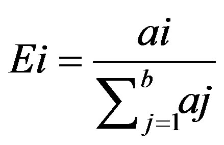
The predicted-to-expected (P/E) ratio was the final evaluation method used to assess model accuracy because it is threshold-independent, it is an assessment of presence-only data, and it can be used to predict several levels of habitat suitability other than just suitable and unsuitable [27]. Ten habitat suitability classes were defined based on the threshold values between zero and one (Table 3). For the P/E curve, ten classes with a class width of 0.1 is the optimum [27]. For each habitat suitability class, the P/E ratio was calculated as
 (14)
(14)
where Pi is the predicted frequency and Ei is the expected frequency [27]. The predicted frequency was calculated as
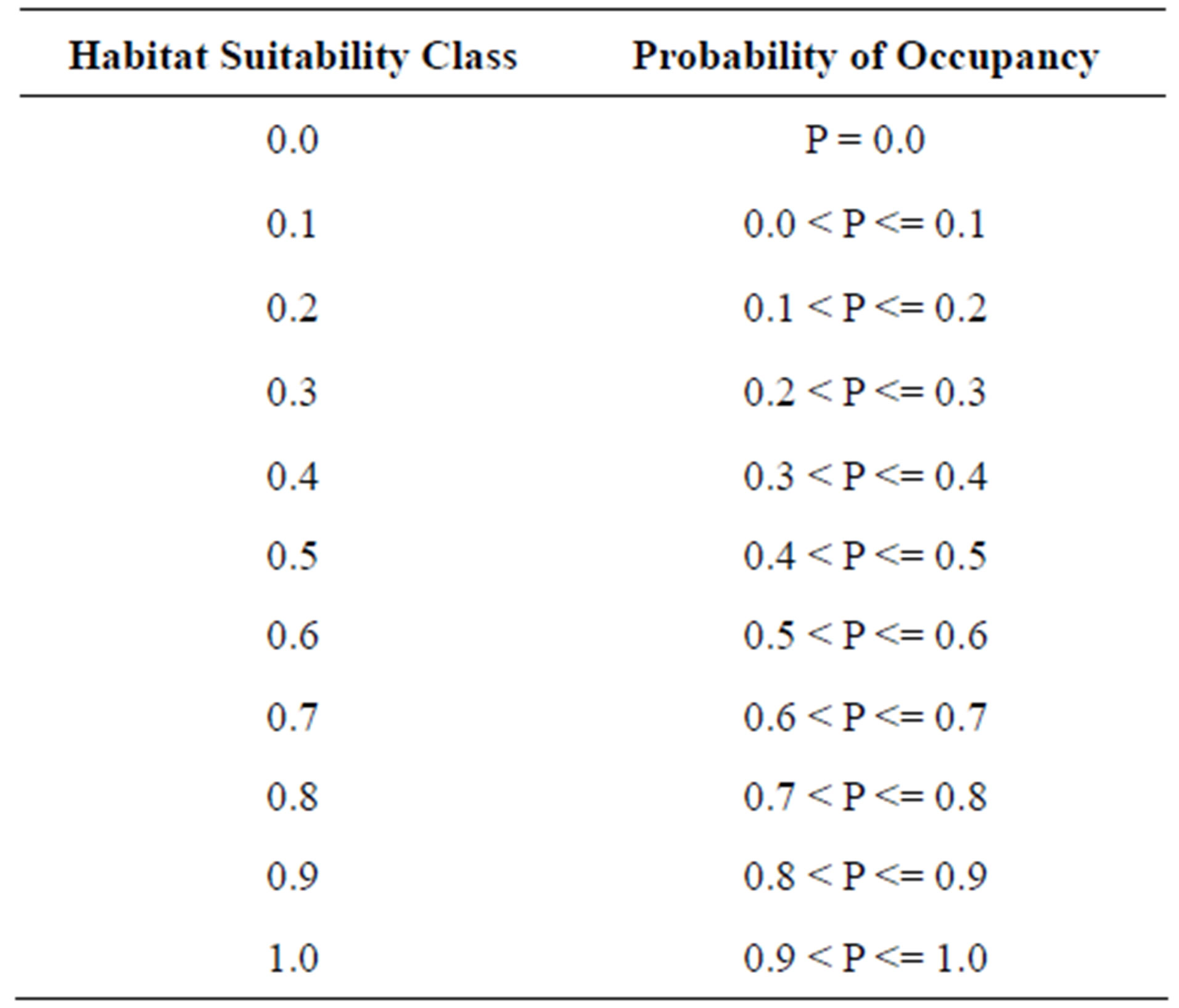
Table 3. Habitat suitability classes defined in the P/E curve. P represents the probability of occupancy for a bare sand patch and varies between zero and one.
 (15)
(15)
where pi is the number of validation data points that fall within the habitat suitability class i and ∑pj is the total number of validation data points [27]. The expected frequency was calculated as
 (16)
(16)
where ai is the area covered by class i and ∑aj is the total area of the study site [27]. In this case, the study site refers to bare sand patches because only habitat is being considered and not total landscape. Fi was plotted against habitat suitability to produce the P/E curve. It is expected that a good model will show a linearly increasing curve with a low suitability class containing fewer presences than expected by chance (Fi < 1) and high suitability classes having Fi increasingly higher than one. A threshold occurs where Fi = 1 below which habitat is unsuitable and above which habitat is suitable [27].
Because the P/E curve did not match what was theoretically expected, k-fold cross-validation was used to assess any biases that may be caused by how the data was used. Hairy prairie-clover presence/absence data was randomly divided into three independent partitions (k = 3) [27]. K-fold cross-validation was applied using two of the partitions to calibrate the model and the left out partition in accuracy assessment, on only the retained variables from the original model [27]. Therefore, two additional evaluations of model accuracy were produced to compliment the original accuracy assessment. Central tendency and variance of the P/E curve were evaluated from the mean, 95% confidence interval, and standard deviation to assess model robustness [27]. The 95% confidence interval was calculated as
 (17)
(17)
where  is the mean and
  is the standard error [25]. Standard error was defined as
 (18)
(18)
where S is the standard deviation and n is the sample size [25]. The standard deviation was calculated as
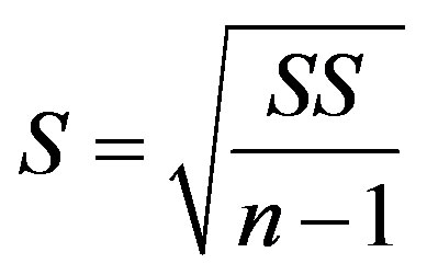 (19)
(19)
where the sum of squares (SS) was defined as
 (20)
(20)
The width of the confidence interval can assess the model’s sensitivity to particular calibration points [27].
Bare sand patches were then re-coded as their predicted habitat suitability based on the probability of occupancy. The habitat suitability threshold for dividing suitable habitat (probability of occupancy above threshold) from unsuitable habitat (probability of occupancy below threshold) was chosen as the threshold value with the highest kappa coefficient, and where the true-positive ratio was maximized and the false-negative ratio was minimized [27]. When choosing the habitat suitability threshold, the goal was to minimize the false-negative ratio so as not to miss valuable hairy prairie-clover habitat. Additionally, four habitat suitability classes were defined from the steps in the P/E curve [27].
3. RESULTS AND DISCUSSION
3.1. Inter-Patch and Intra-Patch Spatial Characteristics for Potential Bare Sand Habitat
Independent-samples t-tests and Mann-Whitney U tests revealed that there was a significant difference between occupied and unoccupied sand patches for most of the variables selected (Table 4). Occupied sand patches were significantly larger in size, more elongated shaped, less isolated, and less vegetated in the early growing season (P < 0.05). There was no significant difference between the NDVI of occupied and unoccupied sand patches in the late growing season (P > 0.05). Therefore, there is no evidence that late season vegetation cover on sand patches significantly affects the occurrence of hairy prairie-clover. Although, there is evidence that vegetation cover on sand patches in the early growing season affects the occurrence of hairy prairie-clover. The mean NDVI in May was significantly lower on occupied sand patches as opposed to unoccupied sand patches (Table 4). Seedling establishment and persistence in the early growing season can be affected by competition for resources with other species, therefore it may be advantageous to hairy prairie-clover to establish on bare sand areas with reduced vegetation cover in the early growing season [3]. As well, different types of vegetation green-up at different times during the growing season, therefore the NDVI in May could be detecting differences in the type of vegetation on sand patches rather than differences in the amount of vegetation. For example, it is commonly observed in the field that juniper inhabits partially to heavily stabilized bare sand areas. Considering juniper is an evergreen shrub it will be captured in the early season NDVI as opposed to species that have not undergone green-up at this time. The difference in NDVI may be capturing the difference in juniper occurrence between sites.
Unoccupied bare sand patches tended to be smaller, more round shaped, more isolated, and more vegetated in the early growing season. Unoccupied sand patches had closer neighbouring sand patches than occupied bare sand areas but, were surrounded by less neighbouring patches. The ENN distance may be a poor measure of isolation because larger patches will have a greater distance between their patch centroids compared to smaller patches. Thus, the value may be an artefact of the measurement and not a true measure of isolation. This also suggests that it is not only the distance between habitat patches but the amount of surrounding habitat that is important to hairy prairie-clover occurrence. Dispersal is mainly affected by patch isolation and matrix quality with small patches being more affected by the quality of the matrix than larger patches [7,8,28]. However, small patches that more densely populate the matrix can influence the nature of the intervening matrix to decrease patch isolation [28]. Therefore, the amount of bare sand habitat within a 30 m proximity of the target patch may be a more ecologically relevant measure of patch isolation than just the ENN distance when considering factors affecting dispersal.
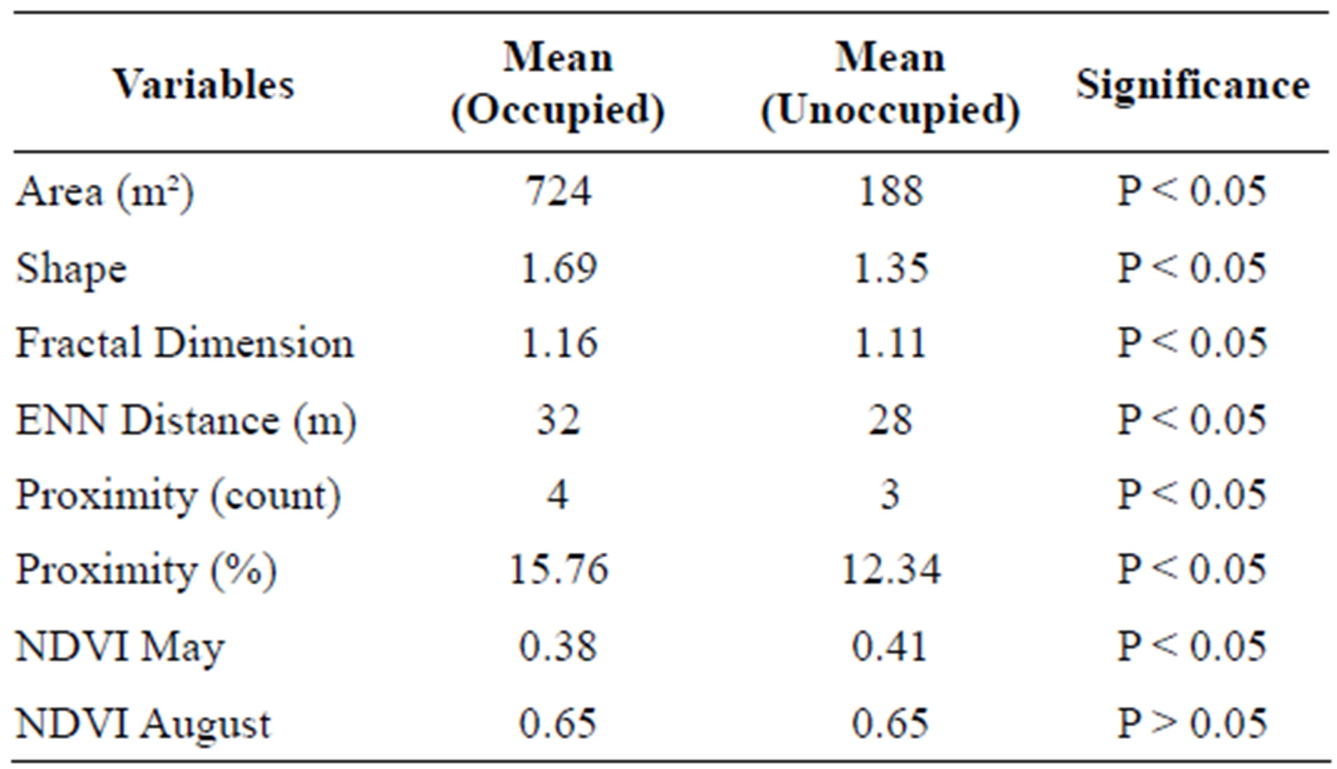
Table 4. Significant differences between occupied and unoccupied sand patches for chosen patch metrics.
3.2. The Spatial Configuration of Hairy Prairie-Clover Habitat
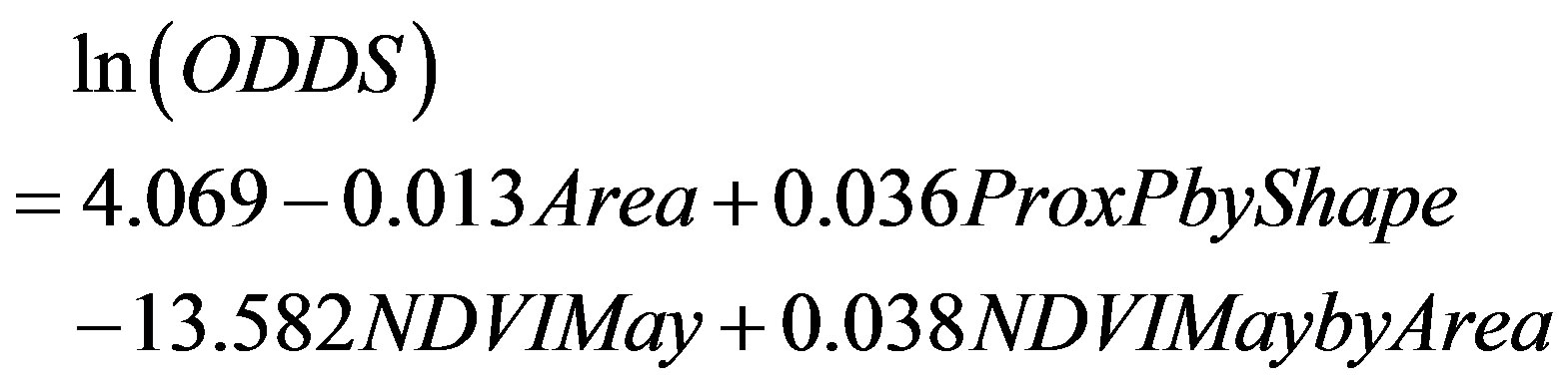
Binary logistic regression revealed that the size and shape of a sand patch, as well as the degree of isolation, and amount of vegetation in the early growing season were significantly correlated with hairy prairie-clover occurrences (Eq.21). Almost 29% of the variation in bare sand patch occupancy could be explained by the logistic regression equation (r² = 0.285 and P < 0.05).
 (21)
(21)
The variable interaction of proximity percent with shape was the most useful for differentiating between occupied and unoccupied sand patches (Table 5). Similarly, other studies have found that the isolation of habitat patches is most important in explaining species richness and community composition because the rescue-effect allows populations to persist in small patches if they are well connected [29]. Adding proximity percent, shape, area, and NDVI May significantly improved the model’s ability to predict suitable and unsuitable bare sand habitat for hairy prairie-clover (Table 5).
Sand patch area and NDVI May could be significant because larger sand patches tend to be less vegetated which decreases the competition for resources with other plants. Biotic interactions between plants act at short distances, but plants are immobile and have limited dispersal, therefore it is advantageous for inferior competitors to occupy competition-free locations [3]. Although some vegetation does take hold on the slipface of large sand dunes, these areas are generally kept clear of vegetation due to wind erosion and lack of soil nutrients and moisture favourable to the growth of most plant species [15], thus providing favourable habitat and competition-free locations for hairy prairie-clover.
Considering that herbivores are one of the major vectors of seed dispersal within the study site [18], proximity percent and sand patch shape can help explain the spatial distribution of hairy prairie-clover. For example,
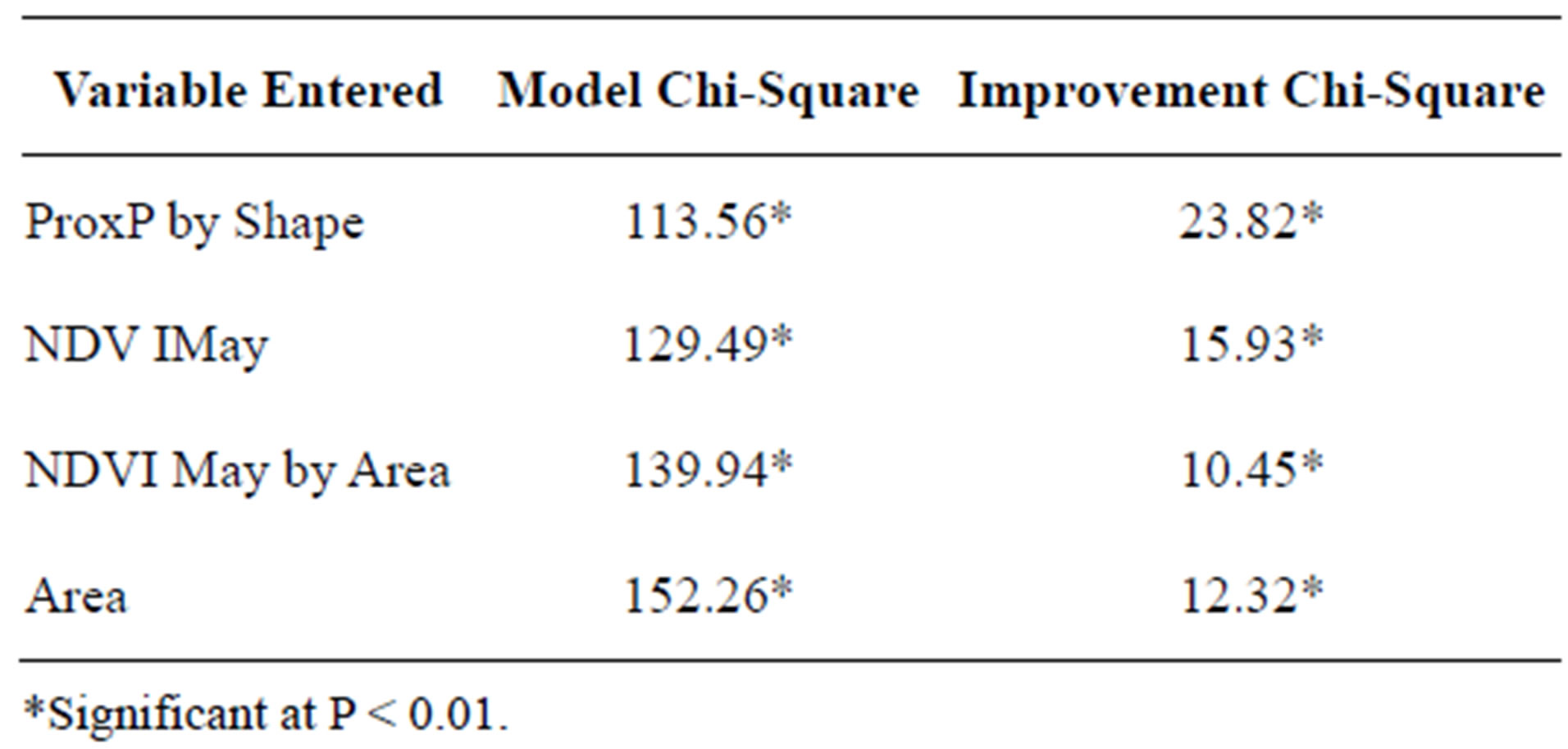
Table 5. Results of logistic regression analysis of variables characterizing occupied and unoccupied sand patches.
ungulates can exhibit specific dispersal behaviour such as the orientation of movement along landscape elements and the ability to choose between patches, which will affect dispersal and exchange rates of seeds between patches [30]. Ungulates, such as white-tailed deer, are more likely to prefer linearly shaped patches because they provide more preferential edge habitat and corridors for movement [31,32]. Thus, the shape of a sand patch could indirectly affect the spatial distribution of hairy prairie-clover through foraging behavior within the landscape. It was found that occupied sand patches were significantly more elongated than unoccupied sand patches (Table 4).
As well, the percentage of the immediate surrounding area (30 m buffer) of a sand patch could indirectly influence the spatial distribution of hairy prairie-clover through its influence on seed dispersal. Dispersal and exchange rates of seeds between patches will flow more readily in well connected patches based on the behavioural rule where individuals will stay at the first patch they reach as opposed to travelling extended distances between patches [30]. Occupied sand patches were also significantly less isolated than unoccupied sand patches (Table 4). Therefore, the spatial distribution of hairy prairie-clover can be explained by three constraints: 1) Patch Area (Area): the local environment allows the population to grow, 2) Patch Quality (NDVI May): interactions with other local species allow the species to persist, and 3) Patch Isolation (ProxP and Shape): the location is accessible given the dispersal abilities of the species [3].
3.3. Habitat Suitability Predictions
The habitat suitability threshold was set at 0.40 because the kappa coefficient was maximized and the sensitivity of prediction was substantially higher than that achieved at a threshold of 0.50 (Table 6 and Figure 2). If the probability of a sand patch being occupied by hairy prairie-clover was equal to or greater than 40%, the sand patch was predicted to be suitable habitat. If the probability of occupancy was less than 40% then the sand patch was predicted to be unsuitable habitat. The goal was to minimize the false-negative ratio by maximizing the sensitivity of predictions. A desirable habitat suitability threshold occurred at 0.40 when considering the risks of over and under predicting suitable habitat (Figure 2). At a threshold value of 0.40, the true-positive ratio is maximized while the false-negative ratio is minimized. At this threshold, 35.5% of the sand patches in the study site were predicted to be suitable hairy prairie-clover habitat and 64.5% were predicted to be unsuitable habitat.
The results of the accuracy assessment for habitat suitability predictions show an average level of model accuracy (Table 6 and Figure 2). The highest kappa value obtained for the logistic regression model was 0.25, indicating a fair level of model agreement with ground referenced data [33]. As well, AUC value at 0.70 indicates an average level of model accuracy [2]. Reference [1] found similar AUC values in their study comparing the accuracy of different species’ distribution models. Across all species in all regions studied and considering only the best methods, they found that 14% of the species had AUC values around 0.70. At the chosen habitat suitability threshold, about 61% of the time the model will correctly predict suitable and unsuitable habitat; about 80% of the time, occurrences are correctly predicted; and about 54% of the time, absences are correctly predicted (Table 6).
3.4. Relationship between Habitat Pattern and Population Pattern
The P/E curve was used to determine threshold values for four habitat suitability classes (Figure 3). A low suitability class should contain fewer evaluation presences than expected by chance (Fi < 1) and high suitability classes should have Fi increasingly higher than 1 [27]. Similar to the results found with the Max Kappa and AUC methods, the habitat suitability threshold for separating suitable habitat from unsuitable habitat occured at 0.40 where the P/E curve crosses the Fi = 1 line (Figure 3). Unsuitable habitat occurred across a probability of
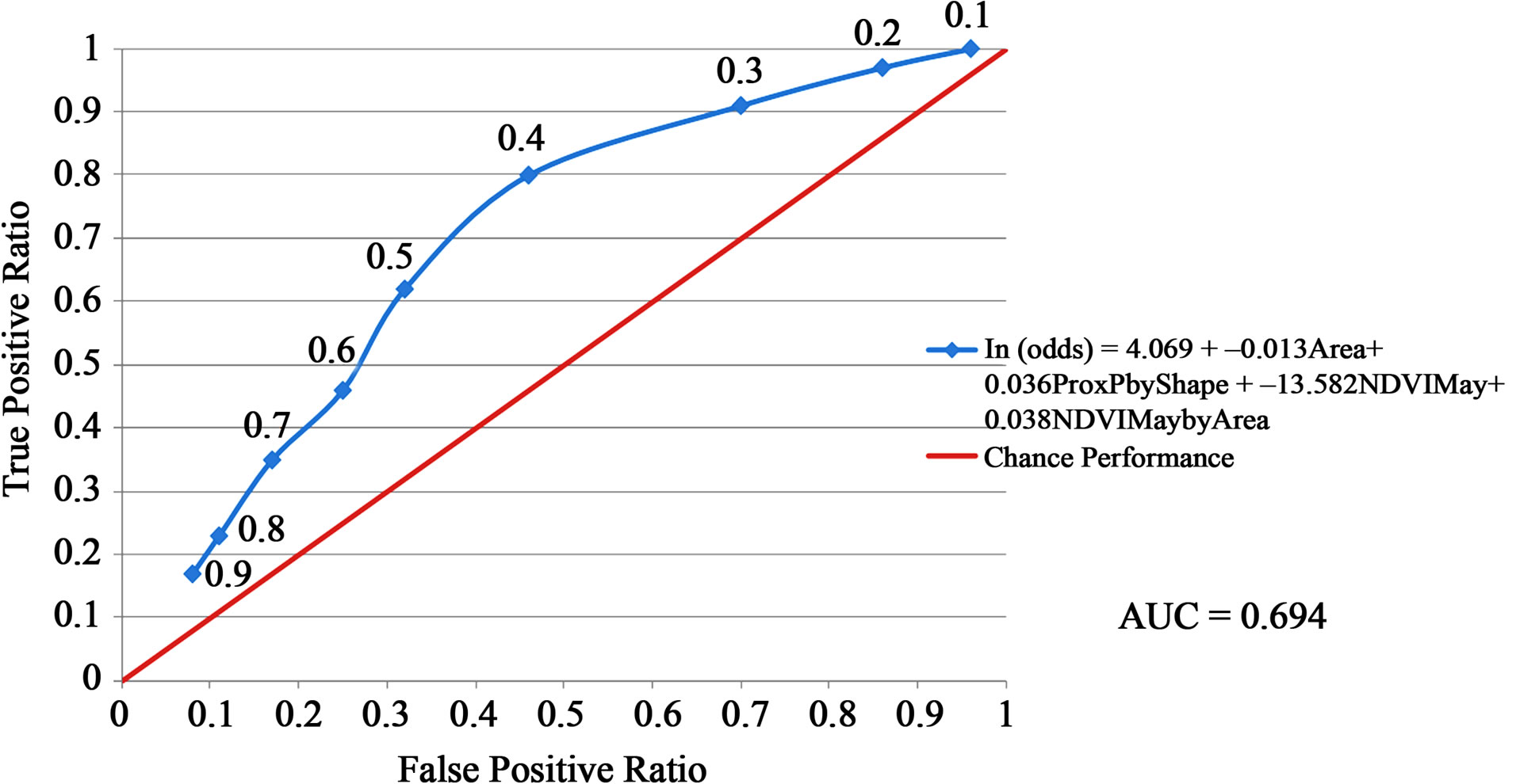
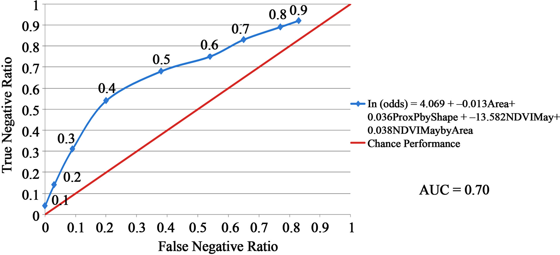
Figure 2. Accuracy assessment of habitat suitability predictions using the Area Under Curve (AUC) method. The red line represents a model that is no better than chance performance and the blue line represents the model derived from the logistic regression equation. The data points on the blue line represent the habitat suitability threshold values as defined in Table 2 .
occupancy less than or equal to 20% where there were fewer evaluation presences than expected by chance (Figure 3). Marginally unsuitable habitat occurred near the transition between suitable and unsuitable habitat at the Fi = 1 line where the number of evaluation presences was close to what would be expected by chance (Figure 3). Suitable habitat occurred where the model predicted the probability of occupancy to be between 40% and 88%, because there were more evaluation presences than expected by chance (Figure 3). Where the model predicted the probability of occupancy to be greater than 88% (marginally suitable), validation data showed that occupancy of these types of sand patches actually dropped off which was not what was theoretically expected to occur (Figure 3).
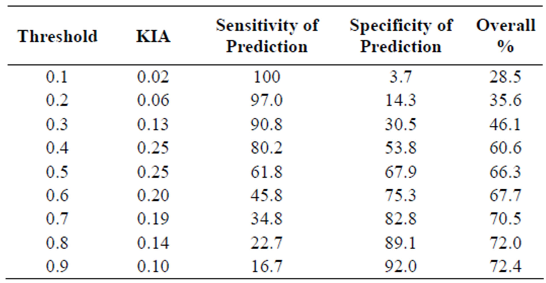
Table 6. Accuracy assessment of habitat suitability predictions using the MaxKappa method. KIA is the kappa coefficient. Threshold values are based on the probability of occupancy as derived from Eq.21. Threshold values are defined in Table 2 .
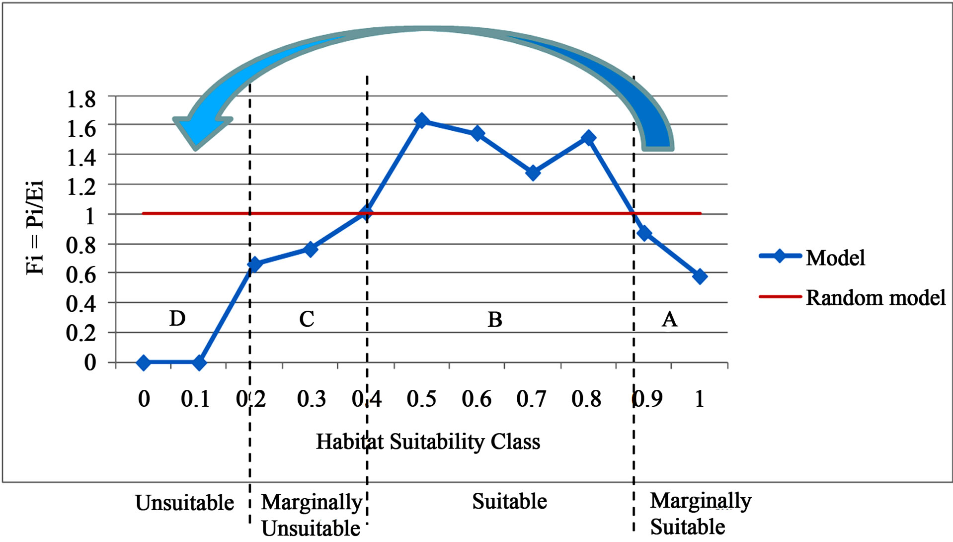
Figure 3.Four habitat suitability classes as derived from the P/E curve. The blue line represents the P/E curve derived from the logistic regression model and the red line represents a chance or random model. Fi is the predicted to expected ratio and the habitat suitability classes are defined in Table 3. The blue arrow represents the direction of natural succession when considering two variables from the logistic regression model: area and NDVI May. (A) Active sand areas (Marginally Suitable habitat: increasing false absences); (B) The transition state of a partially stabilized sand patch (Suitable habitat: mostly true presences); (C) The remnant state of a heavily vegetated sand patch (Marginally Unsuitable habitat: increasing false presences); (D) The altered state with the persistence of a new plant community (Unsuitable habitat: mostly true absences) .
The shape of the P/E curve can be explained by how the logistic regression equation predicts the probability of occupancy. Looking at two variables, NDVI May and area, the model predicts that as sand patches become larger and NDVI May becomes lower the sand patch is more likely to be occupied by hairy prairie-clover (Table 7). Following the shape of the P/E curve, this is true until a threshold is reached around a probability of 0.88 where actual occupancy drops back to being below predicted occupancy. Considering NDVI May and area, natural succession on a sand patch would thus cause the probability of occupancy to decrease as colonizing species stabilize the bare sand area and gradually increase NDVI May and decrease area (Figure 3). This is apparent when looking at the average area and average NDVI May of each habitat suitability class (Table 7).
Landscapes are dynamic rather than static and are in a constant flux of change. The temporal scale of landscape change is different from the temporal scale of flora species’ response to landscape change such that present species occurrences can still reflect past landscape patterns [29,34]. For example, [29] found that current species richness in fragmented alvar grasslands was more significantly related to past areas and connectivities of habitat patches than current habitat pattern. As well, [34] found a significant relationship between present habitat area and current species richness, and habitat area 50 years ago and current species richness in grasslands in south-eastern Sweden. Reference [35] found that remnant patches could exist within a population because there was a considerable time span between migration of new individuals to a patch and the final extinction of species in a patch during succession. Due to the delayed response of plants to habitat change, habitat patches can harbour species that prefer an environment that no longer exists [34]. Therefore, it is not uncommon that hairy prairie-clover was found to occupy marginally suitable habitat and marginally unsuitable habitat in this study.
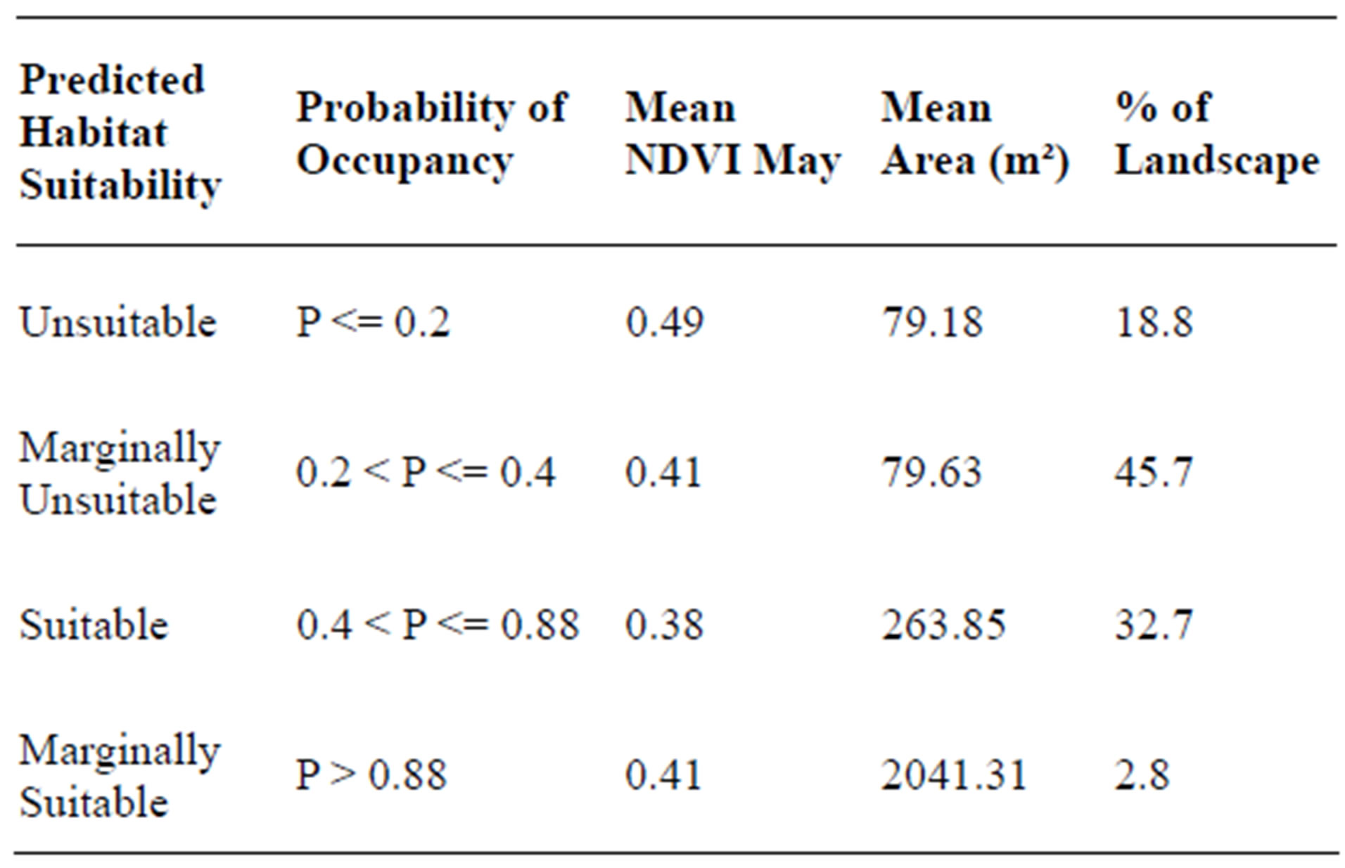
Table 7.The average area and NDVI May of four different habitat suitability classes. As sand patch size increases and NDVI May decreases, the probability of occupancy increases .
Considering the variables present in the logistic regression equation (Table 7) and the shape of the P/E curve, the four habitat suitability classes were derived based on the direction of natural succession (Figure 3). The sand dunes found in the Dundurn area comprise four physiographic categories: active complexes, stabilized blow-outs, stabilized dunes, and dune depressions. When considering three dominant environmental gradients, soil-water holding capacity, edaphic characteristics, and degree of stabilization; stabilized blow-outs and dune depressions have closely related environmental niches while stabilized dunes and active complexes are distinct and follow a distinct environmental gradient between the two. Natural succession reflects the stabilization of active complexes, increasing the water retaining capacity and organic content of sandy soils, towards stabilized dunes. Comparatively, blow-outs represent a more advanced stage of succession due to decreased wind erosion allowing invasion by woody species such as creeping juniper. As well, the more mesic conditions in dune depressions as compared to the exposed slopes of stabilized dunes, allows late successional species to take over and develop a more complex vegetative community [17].
On average, larger sized sand dunes are kept relatively clear of vegetation on their most active surfaces (the dune head, crest, and slip face) due to wind erosion and deposition of sand, and a lack of soil moisture and nutrients preventing growing conditions that are favourable to most species [15]. Active complexes in the Dundurn sand-hills were found to have lower soil organic content, higher percentages of sand, and lower soil moisture [17]. Although these types of sand patches were predicted to have a probability of occupancy greater than or equal to 88% for hairy prairie-clover, accuracy assessment revealed that Fi was less than one (Figure 3(A)). Therefore, these types of sand patches are only marginally suitable and the occurrence of false absences is increasingly higher in these types of sandy areas. False absences occur in these sandy areas because hairy prairie-clover tends to be absent from these potentially suitable sites (Figure 3(A)). While currently they are not preferred habitat, hairy prairie-clover plants are able to colonize them allowing succession to progress towards an environment that is more favourable to the plant.
Hairy prairie-clover prefers to occupy the niche in the successional stage where bare sand areas are partially stabilized (Figure 3(A) and Table 7). Thus, following the environmental gradient along the succession of active complexes to stabilized dunes [17], hairy prairie-clover will be more commonly associated with stabilized dunes than active complexes (Figure 3). Hairy prairie-clover has been found to be positively associated with early invading species of open sand and other early successional species within the Dundurn sand-hills [18]. Sparsely vegetated and frequently disturbed microsites such as partially stabilized sandy areas, favour plants with nitrogen fixing symbiosis because nitrogen fixation provides a net advantage on open, sunny, nitrogen poor sites [9]. Hairy prairie-clover occurrence in sandy areas provides a valuable link in the natural succession of sand dunes and bare sand patches because it is part of the legume family of which most legumes are nitrogen fixers [17].
Hairy prairie-clover has also been found to exist in marginally unsuitable habitat (Figure 3(C)) because nitrogen fixation provides soil nutrients which would otherwise be sparse in a bare sand patch allowing other species to colonize the area. For example, creeping juniper reaches its maximum abundance and is most associated with stabilized blow-outs in the Dundurn sand-hills. The main difference between stabilized dunes and stabilized blow-outs is the higher abundance of creeping juniper in the latter. As well, the most dominant species in dune depressions are Stipa comata and Calamovilfa longifolia which are two species that occur in the later stages of succession [17]. Hairy prairie-clover has been found growing in conjunction with creeping juniper on partially to heavily stabilized sandy areas, even though these sites are not necessarily favourable to the long term persistence of the plant [18]. The biotic interactions that occur with the co-existence of species, especially the existence of a superior competitor (such as the implied relationship between creeping juniper and hairy prairie-clover), will affect the fitness and behaviour of species such that the population will persist as a remnant patch with an extinction debt [3,18,29]. In marginally unsuitable habitats, such as blow-outs and depressions, an increase in false presences is observed. While hairy prairie-clover can occupy marginal habitats, these patches are not necessarily favourable for supporting the long term persistence of the population because natural succession proceeds towards a decrease in habitat suitability for hairy prairieclover.
The standard deviation between the three models from K-fold cross-validation (Figure 4) can help determine which habitat suitability classes were predicted the best and where the model needs improvement [27]. Unsuitable habitat was predicted with relatively high accuracy (Figure 4). The narrowness of the standard deviation shows that all three models in K-fold cross-validation were in agreement for predicted unsuitable hairy prairieclover habitat. As well, suitable habitat was predicted with high confidence as seen in the low variance between the three models from K-fold cross-validation (Figure 4). High variability between model predictions occurred for both marginal habitat types, indicating the models weakness in predicting marginally unsuitable and marginally suitable habitat for hairy prairie-clover. The greatest variation between models occurred at habitat suitabilities
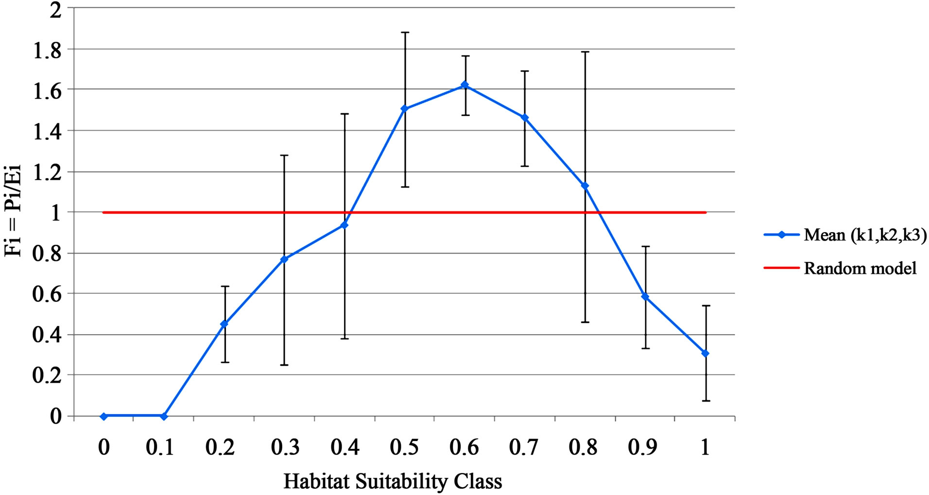
Figure 4.The standard deviation between the three models (K1, K2, K3) from k-fold cross-validation.
of 0.40 and 0.80, at the transition between suitable and unsuitable habitat where the curve crosses the Fi = 1 line (Figure 4). This reflects the model’s inability to account for false presences and false absences.
Considering that the spatial configuration of habitat could explain about 29% of the variation in patch occupancy, it is not surprising that the model was unable to account for false presences and false absences. Including other ecological factors which may influence the occurrence of false presences and false absences could help improve the predictive capability of the model. For example, a study by [2] which included ecological variables such as a topographic wetness index and direct incident solar radiation had an AUC value that was 0.18 higher than that obtained in this study. Variables such as elevation, slope angle, slope aspect, amount of incoming solar radiation, surface soil moisture, and surface wind speed have been identified as key ecological factors affecting population viability in plant species [2,26]. Adding these ecological variables to the model could further explain hairy prairie-clover presence/absence on sand patches.
False presences and false absences occur in populations because species can occupy unsuitable habitat and/ or be absent from suitable habitat. This is due to several reasons, namely 1) the difference in temporal scale between landscape change and flora species’ response to change, and 2) species occupancy can only reflect the realized niche and not the fundamental niche due to abiotic and biotic environmental factors and interactions [3,5,34]. Therefore, the transition between suitable and unsuitable habitat cannot be modelled with high certainty. Further, while statistical methods can determine statistical significance between the mean of a patch metric, ecological significance is harder to detect because many ecological relationships are threshold dependent where only changes in pattern at the threshold are ecologically significant [11]. For example, the extinction of long-lived plants would show an S-shaped curve representing thresholds where the effect on a species suddenly increases. Extinction would progress slowly at the beginning and increase dramatically once a time or area threshold had been reached before levelling out after the extinction debt had been equalized [29,34]. Therefore, hairy prairie-clover can still be found in marginal habitats where successional change has not yet reached a threshold capable of eliciting a response in the plant’s spatial occurrence (Figure 3).
In the final habitat suitability map for hairy prairieclover (Figure 5) almost 46% of the bare sand patches were predicted to be marginally unsuitable hairy prairie-clover habitat, and about 19% of the sand patches were predicted to be completely unsuitable (Table 7). About 33% of the sand patches were predicted to be suitable hairy prairie-clover habitat and only 2.8% were predicted to be marginally suitable (Table 7). Considering the state and transition model of succession in Figure 3, the majority of the bare sand patches in the study site exist as remnant patches undergoing succession. Therefore, there is evidence that in the absence of natural disturbance, the long term trend will be towards a decrease in habitat suitability for hairy prairie-clover.
4. CONCLUSIONS
It has been demonstrated that habitat suitability for hairy prairie-clover can be predicted with an average level of model accuracy (AUC = 0.70 and Max Kappa = 0.25) when only considering factors of habitat spatial pattern. Four significant components of habitat pattern (area, shape, proximity percent, NDVI May) were able to explain almost 29% of the variation in bare sand patch occupancy. Therefore, there is evidence that the spatial configuration of bare sand areas may not be the dominant factor limiting the abundance of hairy prairie-clover on the landscape. Landscape and habitat pattern may not be exerting as much control over population pattern as originally thought.
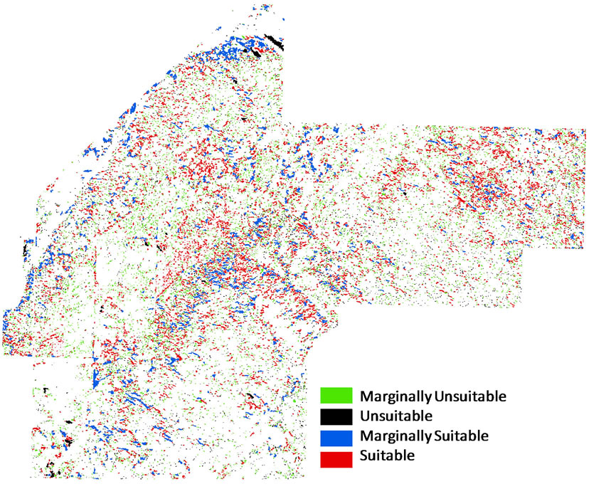
Figure 5.Habitat suitability map for hairy prairie-clover of bare sand patches. The white background consists of classes grassland, shrub, aspen, juniper, and other.
Contrary to what was theoretically expected by the logistic regression model alone, sand patches with a probability of occupancy between 40% and 88% were the most preferred habitat by hairy prairie-clover when crossvalidated with additional occurrence data. It was expected that the model would show a linearly increasing curve as the probability of occupancy increased [27]. Deviation from the theoretical linear curve seen at probabilities greater than about 88% could be a reflection of the time lag between the establishment of a species in an area (marginally suitable habitat with increasing false absences) and the persistence of that species as succession progresses (suitable habitat with true presences). The majority of sand patches in the study site were predicted to be marginally unsuitable and unsuitable hairy prairie-clover habitat. There is evidence that successional trends in the study site are towards a decrease in habitat suitability for hairy prairie-clover. While it appears that current landscape and habitat structure is capable of supporting a large hairy prairie-clover population, the long term persistence of the species’ may be threatened due to progressive formation of remnant patches and possible extinction debts [29]. In the absence of natural disturbance to help maintain successional heterogeneity among sand patches, long term trends will be towards complete stabilization (unsuitable hairy prairie-clover habitat). Therefore, it is important to not only consider the structural component of habitat but the functional and compositional components as well.
5. ACKNOWLEDGEMENTS
The authors are thankful for research funding from the Natural Sciences and Engineering Research Council of Canada, and Environment Canada’s Interdepartmental Recovery Fund. Thank you to the numerous staff and volunteers for help with field surveys.
REFERENCES
- Elith, J., Graham, C., Anderson, R., Dudik, M., Ferrier, S., Guisan, A., Hijmans, R., Huettmann, F., Leathwick, J., Lehmann, A., Li, J., Lohmann, L., Loiselle, B., Manion, G., Moritz, C., Nakamura, M., Nakazawa, Y., Overton, J., Peterson, A., Phillips, S., Richardson, K., ScachettiPereira, R., Schapire, R., Soberon, J., Williams, S., Wisz, M. and Zimmermann, N. (2006) Novel methods improve prediction of species’ distributions from occurrence data. Ecography, 29, 129-151. doi:10.1111/j.2006.0906-7590.04596.x
- Parolo, G., Rossi, G. and Ferrarini, A. (2008) Toward improved species niche modelling: Arnica Montana in the Alps as a case study. Journal of Applied Ecology, 45, 1410-1418. doi:10.1111/j.1365-2664.2008.01516.x
- Hirzel, A. and Le Lay, G. (2008) Habitat suitability modelling and niche theory. Journal of Applied Ecology, 45, 1372-1381. doi:10.1111/j.1365-2664.2008.01524.x
- Freckleton, R. and Watkinson, A. (2002) Large-scale spatial dynamics of plants: Metapopulations, regional ensembles and patchy populations. Journal of Ecology, 90, 419-434. doi:10.1046/j.1365-2745.2002.00692.x
- Williams, J., Seo, C., Thorne, J., Nelson, J., Erwin, S., O’Brien, J. and Schwartz, M. (2009) Using species distribution models to predict new occurrences for rare plants. Diversity and Distributions, 15, 565-576. doi:10.1111/j.1472-4642.2009.00567.x
- Rizkalla, C., Moore, J. and Swihart, R. (2009) Modelling patch occupancy: Relative performance of ecologically scaled landscape indices. Landscape Ecology, 24, 77-88. doi:10.1007/s10980-008-9281-0
- Kindlmann, P. and Burel, F. (2008) Connectivity measures: A review. Landscape Ecology, 23, 879-890.
- Kolb, A. and Diekmann, M. (2005) Effects of life-history traits on responses of plant species to forest fragmentation. Conservation Biology, 19, 929-938. doi:10.1111/j.1523-1739.2005.00065.x
- Leach, M. and Givnish, T. (1996) Ecological determinants of species loss in remnant prairies. Science, 273, 1555-1558. doi:10.1126/science.273.5281.1555
- Fahrig, L. and Merriam, G. (1994) Conservation of fragmented populations. Conservation Biology, 8, 50-59. doi:10.1046/j.1523-1739.1994.08010050.x
- Gustafson, E. (1998) Quantifying landscape spatial pattern: What is the state of the art? Ecosystems, 1, 143-156. doi:10.1007/s100219900011
- Smith, B. (1998) COSEWIC status report on the hairy prairie-clover in Canada. Environment Canada, Ottawa.
- Wolfe, S., Huntley, D. and Ollerhead, J. (1995) Recent and late Holocene sand dune activity in southwestern Saskatchewan. Geological Survey of Canada, Current Research 1995-B, 131-140.
- Vance, R. and Wolfe, S. (1996) Geological indicators of water resources in semi-arid environments: Southwestern interior of Canada. In: Berger, A.R. and Iams, W.J., Eds., Geoindicators: Assessing Rapid Environmental Changes in Earth Systems, A.A. Balkema, Lisse, 251-263.
- Hugenholtz, C. and Wolfe, S. (2005) Recent stabilization of active sand dunes on the Canadian prairies and relation to recent climate variations. Geomorphology, 68, 131-147. doi:10.1016/j.geomorph.2004.04.009
- Thorpe, J. (2007) Saskatchewan rangeland ecosystems, publication 1: Ecoregions and ecosites. Saskatchewan prairie conservation action plan. Saskatchewan Research Council Pub., No.11881-1E07.
- Hulett, G., Coupland, R. and Dix, R. (1966) The vegetation of dune sand areas within the grassland region of Saskatchewan. Canadian Journal of Botany, 44, 1307-1331. doi:10.1139/b66-147
- Godwin, B. and Thorpe, J. (2007) Targeted surveys for plant species at risk in Elbow, Dundurn and Rudy-Rosedale AAFC-PFRA Pastures, 2006. Agriculture and agrifood Canada-prairie farm rehabilitation administration. Saskatchewan Research Council Pub., No. 11997-1E07.
- Environment Canada (2008) National climate data and information archive: Canadian climate normals, 1971-2000. http://_www.climate.weatheroffice.ec.gc.ca/climate_normals
- Canadian Wildlife Service (2004) Species at risk public registery: Canadian distribution of the hairy prairie-clover. http://www.sararegistry.gc.ca/species/speciesDetails_e.cfm?sid=533
- Hirzel, A. and Guisan, A. (2002) Which is the optimal sampling strategy for habitat suitability modelling. Ecological Modelling, 157, 331-341. doi:10.1016/S0304-3800(02)00203-X
- McGarigal, K. and Marks, B. (1995) FRAGSTATS: Spatial pattern analysis program for quantifying landscape structure. General Technical Reports, Portland. Or: U.S. Department of Agriculture, Forest Service, Pacific North- - west Research Station, 122 p.
- Jensen, J. (2005) Introductory digital image processing. 3rd Edition, Prentice-Hall Inc., Upper Saddle River.
- Schleuning, M. and Matthies, D. (2008) Habitat change and plant demography: Assessing the extinction risk of a formerly common grassland perennial. Conservation Biology, 23, 174-183. doi:10.1111/j.1523-1739.2008.01054.x
- Zar, J. (1999) Biostatistical analysis. 4th Edition, Prentice-Hall Inc., Upper Saddle River.
- Wolken, P., Sieg, C. and Williams, S. (2001) Quantifying suitable habitat of the threatened western prairie fringed orchid. Journal of Range Management, 54, 611-616. doi:10.2307/4003592
- Hirzel, A., Le Lay, G., Helfer, V., Randin, C. and Guisan, A. (2006) Evaluating the ability of habitat suitability models to predict species presences. Ecological Modelling, 199, 142-152. doi:10.1016/j.ecolmodel.2006.05.017
- Lord, J. and Norton, D. (1990) Scale and the spatial concept of fragmentation. Conservation Biology, 4, 197-202. doi:10.1111/j.1523-1739.1990.tb00109.x
- Helm, A., Hanski, I. and Partel, M. (2006) Slow response of plant species richness to habitat loss and fragmentation. Ecology Letters, 9, 72-77.
- Heinz, S., Wissel, C. and Frank, K. (2006) The viability of metapopulations: Individual dispersal behaviour matters. Landscape Ecology, 21, 77-89. doi:10.1007/s10980-005-0148-3
- Rieucau, G., Vickery, W., Doucet, G. and Laquerre, B. (2007) An innovative use of white tailed deer (Odocoileus virginianus) foraging behaviour in impact studies. Canadian Journal of Zoology, 85, 839-846. doi:10.1139/Z07-062
- Volk, M., Kaufman, D. and Kaufman, G. (2007) Diurnal activity and habitat associations of white tailed deer in tallgrass prairie of eastern Kansas. Transactions of the Kansas Academy of Science, 110, 145-154. doi:10.1660/0022-8443(2007)110[145:DAAHAO]2.0.CO;2
- Landis, B. and Koch, G. (1977) The measurement of observer agreement for categorical data. Biometrics, 33, 159-174. doi:10.2307/2529310
- Cousins, S., Ohlson, H. and Eriksson, O. (2007) Effects of historical and present fragmentation on plant species diversity in semi-natural grasslands in Swedish rural landscapes. Landscape Ecology, 22, 723-730. doi:10.1007/s10980-006-9067-1
- Eriksson, O. (1996) Regional dynamics of plants: A review of evidence for remnant, source sink and metapopulations. Oikos, 77, 248-258. doi:10.2307/3546063