ABSTRACT

Linear fractional map type (LFMT) nonlinear QCA (NLQCA), one of the simplest reversible NLQCA is studied analytically as well as numerically. Linear advection equation or Time Dependent Schrödinger Equation (TDSE) is obtained from the continuum limit of linear QCA. Similarly it is found that some nonlinear advection- diffusion equations including inviscid Burgers equation and porous-medium equation are obtained from LFMT NLQCA.

Keywords:

Nonlinear Quantum Cellular Automaton, QCA, Quantum Walk, Linear Fractional Map, Advection-Diffusion Equation, Burgers Equation, Porous-Medium Equation, Soliton

1. Introduction

Quantum Cellular Automaton (QCA) [1] is a quantum version of (classical) cellular automaton (CA). The word QCA was introduced by Grössing and Zeilinger [2] . But their model was not completely unitary. The QCA in the right meaning which has both locality and unitarity, was firstly investigated by Meyer [3] [4] [5] [6] , then followed by Boghosian and Taylor [7] [8] , although they used the term Quantum lattice gas automata (QLGA) for the two-component case. Since the middle of the 2000s, new axiomatic approaches of QCA different from previous conventional or ad hoc ones have been proposed by several researchers [9] [10] [11] in order to comprehend QCA in more systematic and unified way by clarifying the definitions and/or to cope with the difficulties for extending it in a form relevant to the infinite dimensional Hilbert space. In most axiomatic QCAs, the unitarity and the causality (namely the existence of the upper limit on the speed of the information propagation) are fundamental and the locality is derived from them [10] . In this study, however, we describe QCA in a rather conventional fashion. There are several frameworks for quantum lattice systems other than QCA, namely Quantum Walk (QW) [12] , Quantum Lattice Gas Automata (QLGA) [7] [8] and Quantum Lattice Boltzmann (QLB) [13] . They are similar or mathematically equivalent to some QCAs [14] [15] [16] .

Consider the simplest partitioned QCA on a 1D-time 1D-space lattice of which time evolution rule is given by Figure 1 and Equation (1). This rule is governed by the 2 × 2 basic unitary matrix (which is called scattering unitary matrix [11] ) which operates on a vector consisting of functions at adjacent grid points.

(1)

The simplest is the QCA with constant U (independent from space and time). We then generalize it to the QCA with space dependent U as described by Equation (2).

(2)

Moreover QCA/QW with time dependent has been studied. Especially remarkable results are obtained for the QW of which parameter is given by Fibonacci sequence [17] [18] . In this paper we propose a non-linear QCA (NLQCA) and investigate its properties. The basic 2 × 2 matrix is given by

(3)

In the NLQCA the basic 2 × 2 matrix depends on the amplitude of wave function. QCA’s fundamental and powerful properties are unitarity, locality, reversibility, and when we construct NLQCA, it is important to keep these properties. NLQCA was investigated by Meyer [19] in a rather general way. And several articles [20] [21] can be found especially in the name of nonlinear quantum walk (NLQW). However it seems that the concrete form of NLQCA has not been presented for the study. We here propose linear fractional map type (LFMT) nonlinear QCA (NLQCA) and study its properties in order to clearly understand NLQCA.

After this introduction, the rest of the article is organized as follows. In Section 2 we introduce LFMT phase rotation and define three typical types of it, type-0, type-1 and type-2. We also perform its fixed point analysis, which is a useful mean to investigate the characteristics of NLQCA. In Section 3 we introduce two kinds of reversible NLQCA using LFMT phase rotation, namely complex-LFMT NLQCA and real-LFMT NLQCA. In Section 4 we investigate the property of complex-LFMT NLQCA focusing on type-0. In Section 5 and 6 we investigate the property of real-LFMT NLQCA (type-0 in Section 5 and type-2 in Section 6).

2. Linear Fractional Map Type Phase Rotation

2.1. Definition

Consider the following map (complex plane to the complex plane itself) which conserves its absolute value.

(4)

or

(5)

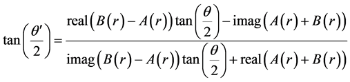
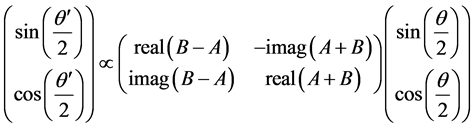
Here are complex numbers and functions of. denotes the complex conjugate of X. As the numerator and the denominator of Equation (4) are complex conjugate with each other, the absolute value of Equation (4) is 1. Therefore Equation (4) represents a phase rotation map. The equivalence of Equations (4) and (5) is proved easily as follows. From Equation (5)

(6)

Then

(7)

It is easily shown that LFMT phase rotations are closed with respect to inversion and composition. (see Equations (44) and (55) in Appendix A)

Generally A, B can be any function of r. However we restrict our discussion to the following 3 cases for simplicity. We discuss type-0 mainly in this study.

(1) type-0

(2) type-1

(3) type-2

Here, are constant complex numbers, and we assume is constant for all cases. There are several formulas on LFMT phase rotations, and we will summarize them in appendix A. We also summarize the extension of this discrete phase rotation to the continuous one in appendix B. Additionally, we use the following notation for simplicity.

[Definition]

denotes the function.

denotes (namely the phase rotation of the double angle of the argument).

For example, by using the above definitions, is simplified

as or.

The function which multiplies the constant k is written as [k]. Note that $ is not included in [] in this case. Complex conjugate operator C, inversion operator V are defined as

(8)

respectively. We will omit the function composition symbol when [..] are uses.

2.2. Small Amplitude Limit and Large Amplitude Limit

In LFMT phase rotation (type-0)

(9)

corresponds to small or large amplitude region respectively.

In small amplitude region this map becomes a linear map and in large amplitude region, this becomes a linear map with complex conjugation. In Figure 2, we illustrate LFMT phase rotation in the case of A = B = 1. We

can see that this map closes to a linear map at the limits of.

2.3. Fixed Points and Their Stability

Approaches from fixed point analysis are useful when we investigate the characteristics of complex-LFMT NLQCA. In general a map from a circle to the circle itself is called a circle map. LFMT phase rotation of Equation (4) is a circle map for any fixed r. Now we find fixed points of this circle map. The equation for the fixed points is

(10)

Apparently the Equation (10) is satisfied when, Namely

(11)

Therefore, Equation (11) has a real solution if and only if. In order to investigate the stability of these fixed points, we calculate the gain of the linearized map around the fixed point. Let x be the small angle deviation from, then we obtain the linearized map as follows.

(12)

This means the phase gain at the fixed point is

(13)

The 2nd equation in the parentheses of Equation (13) is obtained by using Equation (11). If is a fixed point then is another fixed point and it can be proved that the product of the gains for these two fixed points is 1 as shown in Equation (14).

(14)

because the product of the two denominators is

Therefore one fixed point is stable and the other fixed point is unstable or both fixed points are critical (marginally stable/unstable). From Equation (13), the critical situation means, namely or . Moreover, from (11) we can see that in the case and in the case. is merely the lower bound of the condition for a critical point to exist

3. LFMT NLQCA

In this study, we investigate two kinds of NLQCA using LFMT phase rotation. The one is complex-LFMT NLQCA and the other is real-LFMT NLQCA. We refer the Time Dependent Schrödinger Equation (TDSE)-type QCA [22] with additional LFMT phase rotation at each grid point as complex-LFMT NLQCA. And we refer the NLQCA whose basic 2 × 2 unitary matrix (in the sense of Equation (3)) is given by the mapping of real and imaginal part of LFMT phase rotation as real-LFMT NLQCA.

4. Property of Type-0 Complex-LFMT NLQCA

In complex-LFMT NLQCA, the 2 × 2 unitary matrix of linear TDSE- type QCA (see [22] ) and the nonlinear LFMT phase rotation are applied alternatively.

In the above expression is the x-component of Pauli matrices and. In this study, we perform the numerical experiment with

and vary the phase of B. (As the change of the phase of A can be compensated by that of initial value of, we need not vary the phase of A when we investigate merely the qualitative behavior of the time evolution not sensitive to the initial, therefore we set A = 1.) The obtained qualitative behavior of complex-LFMT NLQCA can be summarizes as follows. Before showing the summary of the simulation, we firstly illustrate the region for parameters A, B where a phase lock can occur in Figure 3, which is the key diagram to understand the qualitative behavior. |B| is assumed to be 1 without loss of generality. The unit of horizontal axis is. The region (where a fixed point can exist) is colored blue, although the neighbor of pure imaginal B (namely 0.25, 0.75 in horizontal axis) is left white because both of their fixed points are marginally stable/unstable.

In type-0 LFMT NLQCA, a singular amplitude point exists where. We work on the domain far from such singularity, namely (small amplitude case) and (large amplitude case) in all space and time. We discuss here only small amplitude case. Qualitative behavior is roughly classified by the occurrence of a phase lock.

(Case 1) when imag(B) = 0 [000 in Figure 4]:

Phase lock occurs in all space and the waveform reaches a flat pattern at the end.

(Case 2) when imag(B) is sufficiently small but not 0 [001,999 in Figure 4]:

According to the magnitude relation between, a phase lock or an unlock occurs temporally or spatially. The noise from spatial high frequency is rather low, and the waveform is smooth.

(Case 3) when imag(B) is not small [050,075,100,900,925,950 in Figure 4]:

A phase lock never occurs, and the phase is always rotating.

In Figure 4 we show the snapshots of the waveform at t = 2000. The parameter of the

linear QCA part is, and the parameters of nonlinear phase rotation part are A = 1, |B| = 1 and the arg (B) is varied as.

The 3-digit number DDD in the legend indicates that. Periodic boundary condition is used. At t = 0, is set. Absolute value of two-point averaged are plotted

.

When arg(B) = 0 (Case 0), the perfect phase lock occurs. At

(Case 2), the waveform behaves like an attractive Nonlinear Schrödinger Equation(NLS) (namely it does not diffuse as in free TDSE case) and condensates with a vibration. At

(Case 2), the waveform behaves like a repulsive NLS (namely it

diffuses faster than in free TDSE case). As arg(B) goes away from 0 (Case 3), the waveform behaves like a free TDSE (see 050,075,100,900,925,950) probably because only the time averaged phase rotation speed is mainly effective to the qualitative behavior. Here we

mean NLS by the equation i.

However even in the parameter region of Case 3, singular behaviors are observed at the neighbor of some special parameters which depend also on (the parameter of the linear QCA part). Especially, there is a singular point at

(15)

And above this point (namely) the behavior is significantly different from that of free TDSE. The observation of this phenomena is shown in Figure 5 in

the case of. Moreover other singular points are observed at

(16)

Above these points, the noise level with reference to free TDSE becomes larger. In

Figure 5 periodic boundary condition is used. When

the behavior is perfectly same as free TDSE(see 299) and when it exceed this point, the deviation from the free TDSE occurs (see 300,301,304) and the deviation becomes smaller as arg(B) goes away from the point (see 306,310). In the lower graph (t = 14500) of Figure 5, waveforms of 299,306,310 are almost the same as the initial Gaussian wave-form with a half period’s shift, which is a prominent characteristic of free TDSE. (In general, Hamiltonian all eigenvalue differences of which has a finite common divisor, has temporal periodicity. In free TDSE case, the energy spectrum has the form and has the periodicity time T, and moreover has the pseudo periodicity time T/2. At t = T/2, only the n = odd components change their sign, which means the half spatial period’s shift of any initial waveform.) Note that with respect to free TDSE t = 2750

of Figure 5 approximately corresponds to t = 2000 of Figure 4,

because. We need further investigation on the state

and the mechanism of these singularities.

5. Property of Type-0 Real-LFMT NLQCA

5.1. Parameters for the Numerical Experiment

From this section we investigate real-LFMT NLQCA. Firstly we explain the parameters A, B we use in the case of type-0 described by Equation (17).

(17)

As, we have only to investigate 32 out of 64 (= 8 × 8) parameter sets, and moreover about a half of those 32 is sufficient if we employ the space reflection symmetry (P) which we explain next.

5.2. Symmetry and Classification

We consider the following CPTA symmetry (Equations (18)-(21)). We find that the NLQCAs with a parameter which belongs to the same parameter groups behave qualitatively similarly.

・ C-inversion (see Equations (45) and (46) in Appendix A)

(18)

・ P-inversion (see Equations (45) and (46) in Appendix A)

(19)

(Note that, namely [i] C means P-inversion which swaps a and b.)

・ T-inversion (see Equation (44) in Appendix A)

(20)

・ A-inversion (see Equation (45) in Appendix A)

(21)

These C, P, T, A have the following properties.

(1) (namely involution)

(2) A commutes with P, T, C

(3) P commutes with T (PT = TP)

(4) C “anti”-commute with T, P (CP = PCA, CT = TCA)

We define the 6 groups C, D, E, F, G, H so that ID1 and ID2 belongs to the same group if ID1 and ID2 can be transformed each other by C, P, T, A. IDs that belongs to the same group have qualitatively similar behaviors.

[Remark]

These symmetry formulas are same for the type-2, because A, B can be regarded as function of |$| and we can replace A with in Equations (18)-(21).

The CPTA mapping for ID = (n, m) of Equation (17) is shown in Table 1.

As illustrated in Figure 6, C-inversion is simply a redefinition of the sign of the amplitudes. A-inversion is also redefinition of the sign (in this case sign inversion of the all amplitudes).

5.3. Type-G (50/10), Type-E (70), Type-C (60)

In this section we show simulated waveform of type-G/E/C. For these cases, evolution of the waveform can be explained almost by comparing to the corresponding continuous time counterpart equation we discuss later. In Figure 7 and Figure 8 the simulated waveforms of type-G are shown. In Figure 9 the simulated waveform of type-E is shown. In Figure 10 the simulated waveform of type-C is shown. In all cases initial (t =

0) waveform is set to the Gaussian form and

simulated both in forward time (blue) and backward time (red) with a periodic boundary condition. Backward time evolution is performed using T-inversion formula (20).

Two-point-averaged are plotted and the spatial axis indicates.

Type-G (Figure 7) corresponds to the in viscid Burgers equation, where T-inversion simply corresponds to the inversion of moving direction. After the steep slope collapses, the NLQCA waveform goes out of the applicable range of in viscid Burgers equation approximation and KdV’s soliton-like wave packets spawn (see Figure 8).

In type-E (Figure 9) we can observe very slow diffusive behavior. This can be approximated by the certain kind of non-linear diffusion equation which we discuss later. In backward time simulation the sign of the amplitude is inverted at the beginning then behaves as a non-linear diffusion equation. This initial amplitude inversion behavior can be interpreted as the transition process from the non-positive diffusion constant to the positive one.

Type-C (Figure 10) lies between type-G and type-E and behaves like a Burgers equation with viscosity, namely the steep slope does not collapse and keeps on moving with lowering its height. In backward time simulation the sign of the amplitude is inverted at the beginning as in type-E then behaves like a viscid Burgers equation.

5.4. Type-H (51), Type-F (71), Type-D (61)

In this section we show that type-F and type-H can be understood from the view point of fixed point. In the case of real-LMFT NLQCA the meaning of a fixed point is slightly different from that in the case of complex-LMFT NLQCA we discussed before. In this case, a fixed point waveform does not keep still but propagates to ±45 deg. direction in the spacetime. Now we consider the (pseudo) fixed point equation for a fixed waveform moving to the left or right at the speed of one. Namely

(22)

or equivalently using,

(23)

Here means a true fixed point or a pseudo fixed point respectively, and “pseudo” means accepting temporal sign alternation.

As

(from Equations (45) (46) (48) in Appendix A), Equation (23) can be rewritten as

(24)

Obviously, in order for z to be a true fixed point or a pseudo fixed point, must be

(25a)

(25b)

where R, I denotes the set of real numbers and the set of pure imaginary numbers respectively. Sufficient (and presumably necessary) conditions for Equation (25) are

(26a)

(26b)

Namely, using Equation (24)

(27a)

(27b)

From Equation (17) and Table 1, we conclude that type-F has true fixed points, and type-H has pseudo fixed points.

In Figure 11, Figure 12, Figure 13, simulated waveforms of type-H, type-F, type-D are shown respectively. In all cases initial (t = 0) waveform is set to the Gaussian form

and simulated both in forward time (blue)

and backward time (red) with a periodic boundary condition. Backward time evolution is performed using T-inversion formula (20). Two-point-averaged are plotted

and the spatial axis indicates x/2. In all cases

waveforms around the start time, after a short time (t = 9900 to 10100) and after a long time (t = 499900 to 500100) are shown. Type-H (Figure 11) is half stable and Type-F (Figure 12) is super-stable and Type-D (Figure 13) is unstable. These results correspond to the above fixed point analysis. In these simulations we used

the NLQCA parameter in all cases therefore in the small amplitude limit the phase rotation becomes. This corresponds to the

advection type linear QCA with advection speed where the time evolution of the waveform is described as the superposition of the left-moving and right- moving wave packets (see [22] ). In this case,

component moves right with temporal sign alternation, and component moves left with a constant sign. (corresponds to and corresponds to in Equation (27) respectively.)

In type-H (Figure 11) two mountain-shaped wave packets move to opposite directions. The right-moving wave packet (which corresponds to the pseudo fixed point) is stable forever whereas the left-moving wave packet becomes unstable in the long run. Here only the waveforms for even t are plotted, therefore the temporal sign alternation of the right-moving wave packet cannot be seen. In type-F (Figure 12) the right-mov- ing wave packet disappears soon whereas the left-moving wave packet (which corresponds to the true fixed point) is super-stable. In type-D (Figure 13) the waveform is similar to type-F, namely the right-moving wave packet disappears soon whereas the left-moving wave packet keeps moving. However this left-moving wave packet becomes unstable in the long run.

5.5. Continuum Limit of Type-0 Real-LFMT NLQCA

It is known that the continuum limit of the simplest QCA becomes linear advection equation or TDSE (see for example [22] ). We find that in the case of type-0 real-LFMT NLQCA the continuum limit becomes a nonlinear advection-diffusion equation. Concretely, in type-0 real-LFMT NLQCA, the continuum limit exists if B is real. Consider the case where the velocity depends on the amplitudes (a, b, c, d) in the advection type QCA (see for example [22] ).

(28)

As is the average of the amplitude and is the difference

between the right side average and the left side average, p and (q/2) means the coeffi-

cients of ψ and in. Let be respectively then we have

(29)

By inserting Equation (28) to Equation (29) we have

(30)

Therefore

(31)

As Equation (31) implies that, we thus obtain the type-0 real- LFMT NLQCA

(32)

As NLQCA is unitary, its continuum limit must be unitary time evolution equation. The best candidate is

(33)

Note that the operators are anti-Hermite.

Equation (33) can also be rewritten in the following forms.

(34)

or if we set

(35)

This implies is a conserved quantity. We can regard this equation as nonlinear advection diffusion equation of which advection coefficient and diffusion coefficient are proportional to. When p = 0 this type of nonlinear diffusion equation is called as a porous-medium equation [21] [23] . (In this case for Equation (35) the degree of the

porosity). In the article [21] a certain kind of NLQW was proposed and it was

shown numerically that its continuum limit obeys a porous-medium equation with the degree of the porosity approximately 1.5.

In Figure 14, we demonstrate using numerical simulation that the continuum limit of NLQCA of Equation (32) is indeed well described by Equation (33). The PDE (33) is solved using Finite Difference Method (FDM) (Runge-Kutta (4th order)). Real PDE parameters are taken from A using Equation (32).

6. Property of Type-2 Real-LFMT NLQCA

6.1. Relation to TDSE-Type Linear QCA

Type-2 real-LFMT NLQCA is related to type-0 real-LFMT NLQCA with a space inversion (see Equation (48) in Appendix A) and the basic 2 × 2 matrix of type-2 real LFMT NLACA becomes the form of Equation (36) in small amplitude limit.

(36)

The linear QCA governed by Equation (36) is related to the TDSE-type linear QCA of which basic 2 × 2 matrix is given by Equation (37).

(37)

Both linear QCAs (Equations (36) and (37)) have essentially the same dispersion relation Equation (38) and basically behave as TDSE [22] .

(38)

Note that according to the argument in [22] , the 2 × 2 unitary matrices in the Z- transformation representation for Equations (36) and (37) are

(39)

And the eigenvalues of and have essentially the same value except the constant phase factor, which leads to Equation (38). However in the limit,

eigenvectors of are, whereas eigenvectors of are. Therefore the linear QCA governed by Equation (36) (which does not have eigenvector) is thought to be described by the superposition of two (something like “forward going” and “backward going” corresponding to) TDSEs in the wavenumber

limit just like the advection type linear QCA (see [22] ). Now we assume the form of Equation (40) as in the case of type-0 NLQCA (Equations (28) (29)) expecting to obtain type-2 NLQCA.

(40)

However this time is expressed as Equation (41), not in a rational form.

(41)

It is not straightforward to represent type-2 real-LFMT NLQCA using continuum limit approach as in the case of type-0 NLQCA.

6.2. Relation between Type-2 Large Amplitude and Type-0 Small Amplitude

In this section, we try to understand the large amplitude behavior of type-2 NLQCA by relating it to the small amplitude behavior of type 0. Using both-sides inversion and

conjugation formula ((54) in Appendix A), we can state that if z evolves by type-0 NLQCA then evolves by type-2 NLQCA. So if obeying type-0 NLQCA varies slowly in space, and its continuum limit is some PDE for, then the continuum limit of type-2 NLQCA is expected to become approximately the PDE rewritten for.

(Note that it is important to consider the pair not of but of. Using means using

for the adjacent grid points pair which causes sign alternating behavior of.)

We numerically examine the validity of the approximation in the case of inviscid Burges equation. Inviscid Burgers case (type-G) is the most promising for the above

continuum limit argument to be applicable because the PDE for is unitary time

evolution too. (This can be easily verified by the fact that the flux in Equation (35) contains only.)

In Figure 15, we show the simulated NLQCA waveforms of both for

and for. Two waveforms match

well, although a certain adjusting parameter need to be introduced.

Note that we do not plot the solution of the inversed Burgers equation itself but plot its inverted values. Initial waveform for Burgers equation is

and its inverse is used for the inversed Burgers equation.

7. Conclusion

Linear fractional map type (LFMT) nonlinear QCA (NLQCA), is studied analytically as well as numerically. Firstly we introduce LFMT phase rotation which maps the complex plane to itself conserving its absolute value. We employ this LFMT phase rotation in

two ways in order to construct reversible NLQCA, namely complex-LFMT NLQCA and real-LFMT NLQCA. In order to categorize the qualitative behavior of the LFMT NLQCA, stability analysis around fix points is introduced. Complex- and Real-LFMT NLQCA are studied numerically using a simple model. Results are summarized and analyzed according to the category by the symmetry classification for real-LFMT NLQCA. We further study the continuum limit of the real-LFMT NLQCA analytically and verify it numerically. Linear advection equation or Time Dependent Schrödinger Equation (TDSE) is obtained from the continuum limit of linear QCA. Similarly it is found that nonlinear advection-diffusion equations including inviscid Burgers equation and porous-medium equation are obtained from real-LFMT NLQCA. Although it is already reported in the article [21] the emergence of this porous-medium equation as the continuum limit of some NLQW, real-LFMT NLQCA in our study includes more general dynamics. We also observe soliton-like behavior.

Acknowledgements

This research was supported by TUT Programs on Advanced Simulation Engineering, Toyohashi University and University-Community Partnership promotion center, Toyohashi University. We would like to thank Prof. Hitoshi Goto for his support.

Cite this paper

Hamada, S. and Sekino, H. (2016) Solution of Nonlinear Advection-Diffusion Equations via Linear Fractional Map Type Nonlinear QCA. Journal of Quantum Information Science, 6, 263- 295. http://dx.doi.org/10.4236/jqis.2016.64017

References

Appendix A: Formulas on LFMT Phase Rotation

As mentioned in 2.1, and denotes the function

Scale transformation

(42)

Inverse transformation

(43)

By clearing the fraction of the left equation and replacing zz* with z'z'* the right equation is obtained. Namely

(44)

is obtained.

Rotation

(45a)

(45b)

(45c)

(45d)

Here A, B are constants, or A, B can be functions of |$| if |k| = 1.

[Proof]

Equation (45a) is the special case of the general formula. Equation (45b) is obvious from

(Note that the factor u(k) must be factored out to the left, or $ (=evaluated value of the right side) would be changed.)

Equations (45c) and (45d) can be obtained from Equations (45b) and (45a) respectively by applying C from the right and using Equation (48). Note that if |k| = 1 Equations (45c) and (45d) can be obtained also by replacing A with in Equations (45a) and (45b).

Both sides conjugation

(46)

A, B can be a function of |$|.

[Proof]

(47)

Right side conjugation

(48)

A, B can be a function of |$|. This formula means that type-0 LFMT phase rotation is related to type-2 LFMT phase rotation via complex conjugation (C).

[Proof]

(49)

[Remark]

A, B can be a function of |$|. Therefore especially for type-1 and type-2

(50a)

(50b)

are satisfied.

Left side conjugation

(51)

Note that the left side conjugation is equivalent to the both sides inversion if A and B are swapped (see Equation (52)). A, B can be a function of |$|.

[Proof]

It is obvious by applying the right side conjugation formula then the both side inversion formula.

Both side inversion

(52)

[Proof]

(53)

Both side inversion and conjugation

(54)

It is easily derived from both side inversion and both side conjugation formulas. Different from conjugation formula, A, B cannot be regarded as a general function of |$| in (52)-(54).

Composition of mappings

(55)

As A, B, A', B' are functions of |$|, it is closed. Especially for type-1

(56)

Therefore it is closed even when A, B, A', B' are restricted to fixed complex number.

Appendix B: Continuous Time Version on LFMT Phase Rotation

Here we discuss extension of the discrete time LFMT phase rotation to the continuous time LFMT phase rotation. This discussion may be the foundation for the more complicated problem such as the continuum limit of the complex-LFMT NLQCA. It is well known that infinitesimal LFM is governed by Riccati-type equation [24] .

Consider the differential equation for

(57)

By integrating for unit time, we obtain LFMT phase rotation.

(58)

Here A, B can be a function of |z|.

[Proof]

Assume that the continuous time extension of (58) obeys the following differential equation Equation (59) in the polar coordinate.

(59)

Let then using

(60)

We have the following Riccati equation.

(61)

Riccati equation can be linearized by setting

(62)

And the time evolution is expressed as follows.

(63)

By setting

(64)

and using the relation (I: unit matrix),

(65)

is obtained. Therefore the time evolution of is expressed in the form of LFM as follows.

(66)

By comparing with Equation (5), (written again here as Equation (67))

(67)

We have

(68)

Reversely (a, b, c) can be obtained from (A, B) by using

(69)

as

(70)

From this and setting, we have the goal equation Equation (57).

[Remark]

The point where is not singular. True singular point is only

the point where. The condition is the condition that there is no fixed point. (namely phase is always circulating). In the case of,

we use and both and are pure imaginal then a, b, c are real. Although (namely multivalued) when real (B)

= 0, the sign does not affect the integrated result.

Submit or recommend next manuscript to SCIRP and we will provide best service for you:

Accepting pre-submission inquiries through Email, Facebook, LinkedIn, Twitter, etc.

A wide selection of journals (inclusive of 9 subjects, more than 200 journals)

Providing 24-hour high-quality service

User-friendly online submission system

Fair and swift peer-review system

Efficient typesetting and proofreading procedure

Display of the result of downloads and visits, as well as the number of cited articles

Maximum dissemination of your research work

Submit your manuscript at: http://papersubmission.scirp.org/

Or contact jqis@scirp.org

References

- 1. Wiesner, K. (2009) Quantum Cellular Automata. Encyclopedia of Complexity and Systems Science, Springer, New York, 7154-7164.
https://doi.org/10.1007/978-0-387-30440-3_426 - 2. Grössing, G. and Zeilinger, A. (1988) Quantum Cellular Automata. Complex Systems, 2, 197-208.
- 3. Meyer, D.A. (1996) From Quantum Cellular Automata to Quantum Lattice Gases. Journal of Statistical Physics, 85, 551–574.
https://doi.org/10.1007/BF02199356 - 4. Meyer, D.A. (1997) Quantum Mechanics of Lattice Gas Automation: One Particle Plane Waves and Potential. Physical Review E, 55, 5261-5269.
https://doi.org/10.1103/PhysRevE.55.5261 - 5. Meyer, D.A. (1998) Quantum Mechanics of Lattice Gas Automata: Boundary Conditions and Other Inhomogeneities. Journal of Physics A, 31, 2321-2340.
https://doi.org/10.1088/0305-4470/31/10/009 - 6. Meyer, D.A. (1997) Quantum Lattice Gasses and Their Invariants. International Journal of Modern Physics C, 8, 717-735.
https://doi.org/10.1142/S0129183197000618 - 7. Boghosian, B.M. and TaylorI, V.W. (1998) Quantum Lattice-Gas Model for the Many-Par-ticle Schrödinger Equation in D Dimensions. Physical Review E, 57, 54-66.
https://doi.org/10.1103/PhysRevE.57.54 - 8. Boghosian, B.M. and TaylorI, V.W. (1998) Simulating Quantum Mechanics on a Quantum Computer. Physica D, 120, 30-42.
https://doi.org/10.1016/S0167-2789(98)00042-6 - 9. Schumacher, B. and Werner, R. (2004) Reversible Quantum Cellular Automata.
- 10. Arrighi, P., Nesme, V. and Werner, R. (2011) Unitarity Plus Causality Implies Localizability. Journal of Computer and System Sciences, 77, 372-378.
https://doi.org/10.1016/j.jcss.2010.05.004 - 11. Arrighi, P. and Grattage, J. (2012) Partitioned Quantum Cellular Automata Are Intrinsically Universal. Journal of Natural Products, 11, 13-22.
https://doi.org/10.1007/s11047-011-9277-6 - 12. Venegas-Andraca, S.E. (2012) Quantum Walks: A Comprehensive Review. Quantum Information Processing, 11, 1015-1106.
https://doi.org/10.1007/s11128-012-0432-5 - 13. Succi, S. and Benzi, R. (1993) Lattice Boltzmann Equation for Quantum Mechanics. Physica D: Nonlinear Phenomena, 69, 327-332.
https://doi.org/10.1016/0167-2789(93)90096-J - 14. Succi, S., Fillion-Gourdeau, F. and Palpacelli, S. (2015) Quantum Lattice Boltzmann Is a Quantum Walk. EPJ Quantum Technology, 2, 12.
https://doi.org/10.1140/epjqt/s40507-015-0025-1 - 15. Hamada, M., Konno, M. and Segawa, E. (2005) Relation between Coined Quantum Walks and Quantum Cellular Automata. RIMS Kokyuroku, 1422, 1-11.
- 16. Shakeel, A. and Love, P.J. (2013) When Is a Quantum Cellular Automaton (QCA) a Quantum Lattice Gas Automaton (QLGA)? Journal of Mathematical Physics, 54, Article ID: 092203.
https://doi.org/10.1063/1.4821640 - 17. Ribeiro, P., Milman, P. and Mosseri, R. (2004) Aperiodic Quantum Random Walks. Physical Review Letters, 93, Article ID: 190503.
https://doi.org/10.1103/physrevlett.93.190503 - 18. Di Molfetta, G., Honter, L., Luo, B.B., Wada, T. and Shikano, Y. (2015) Massless Dirac equation from Fibonacci Discrete-Time Quantum Walk. Quantum Studies: Mathematics and Foundations, 2, 243-252.
https://doi.org/10.1007/s40509-015-0038-6 - 19. Meyer, D.A. (1996) Unitarity in One Dimensional Nonlinear Quantum Cellular Automata.
- 20. Navarrete-Benlloch, C., Pérez, A. and Roldán, E. (2007) Nonlinear Optical Galton Board. Physical Review A, 75, Article ID: 062333.
https://doi.org/10.1103/physreva.75.062333 - 21. Shikano, Y., Wada, T. and Horikawa, J. (2014) Discrete-Time Quantum Walk with Feed-Forward Quantum Coin. Scientific Reports, 4, 4427.
https://doi.org/10.1038/srep04427 - 22. Hamada, S., Kawahata, M. and Sekino, H. (2013) Solution of the Time Dependent Schrödinger Equation and the Advection Equation via Quantum Walk with Variable Parameters. Journal of Quantum Information Science, 3, 107-119.
https://doi.org/10.4236/jqis.2013.33015 - 23. Vazquez, J.L. (2006) The Porous Medium Equation, Mathematical Theory. Oxford University Press, Oxford.
https://doi.org/10.1093/acprof:oso/9780198569039.001.0001 - 24. Hlavaty, L., Steinberg, S. and Wolf, K.B. (1984) Riccati Equations and Lie Series. Journal of Mathematical Analysis and Applications, 104, 246-263.
https://doi.org/10.1016/0022-247X(84)90046-5