Open Journal of Statistics
Vol.4 No.7(2014), Article
ID:49306,9
pages
DOI:10.4236/ojs.2014.47049
Application of Sparse Bayesian Generalized Linear Model to Gene Expression Data for Classification of Prostate Cancer Subtypes
Behrouz Madahian1, Lih Y. Deng1, Ramin Homayouni2,3
1Department of Mathematical Sciences, University of Memphis, Memphis, TN, USA
2Bioinformatics Program, University of Memphis, Memphis, TN, USA
3Department of Biology, University of Memphis, Memphis, TN, USA
Email: bmdahian@memphis.edu, lihdeng@memphis.edu, rhomayoun@memphis.edu
Copyright © 2014 by authors and Scientific Research Publishing Inc.
This work is licensed under the Creative Commons Attribution International License (CC BY).
http://creativecommons.org/licenses/by/4.0/


Received 8 June 2014; revised 11 July 2014; accepted 20 July 2014
Abstract
A major limitation of expression profiling is caused by the large number of variables assessed compared to relatively small sample sizes. In this study, we developed a multinomial Probit Bayesian model which utilizes the double exponential prior to induce shrinkage and reduce the number of covariates in the model [1] . A hierarchical Sparse Bayesian Generalized Linear Model (SBGLM) was developed in order to facilitate Gibbs sampling which takes into account the progressive nature of the response variable. The method was evaluated using a published dataset (GSE6099) which contained 99 prostate cancer cell types in four different progressive stages [2] . Initially, 398 genes were selected using ordinal logistic regression with a cutoff value of 0.05 after Benjamini and Hochberg FDR correction. The dataset was randomly divided into training (N = 50) and test (N = 49) groups such that each group contained equal number of each cancer subtype. In order to obtain more robust results we performed 50 re-samplings of the training and test groups. Using the top ten genes obtained from SBGLM, we were able to achieve an average classification accuracy of 85% and 80% in training and test groups, respectively. To functionally evaluate the model performance, we used a literature mining approach called Geneset Cohesion Analysis Tool [3] . Examination of the top 100 genes produced an average functional cohesion p-value of 0.007 compared to 0.047 and 0.131 produced by classical multi-category logistic regression and Random Forest approaches, respectively. In addition, 96 percent of the SBGLM runs resulted in a GCAT literature cohesion p-value smaller than 0.047. Taken together, these results suggest that sparse Bayesian Multinomial Probit model applied to cancer progression data allows for better subclass prediction and produces more functionally relevant gene sets.
Keywords:LASSO, Robustness, Sparsity, MCMC, Gibbs Sampling

1. Introduction
As data collection technologies evolve, the number of covariates which can be measured in experiments increase. For example, modern microarray experiments can measure the expression levels of several thousand genes simultaneously. Since the number of samples is typically much smaller than the number of covariates, it is challenging to identify important genes among the large amount of data points [4] . Many univariate analysis approaches have been applied to select important genes from microarray experiments such as t-test [5] , regression modeling [6] , mixture model [7] and non-parametric methods [8] [9] . However, since most complex traits are polygenic, a single variable analysis can only detect a very small portion of the relevant variation and may not be powerful enough to identify weaker interactions between the variables [10] .
In order to address limitations of single covariate analysis methods, several approaches have been developed for simultaneous analysis of multiple covariates [11] -[13] . In linear regression framework, the least square method is used to obtain estimate of parameters. The ordinary least square estimates obtained are not quite satisfactory mainly due to poor accuracy of prediction resulting from high variances of estimates and the large number of covariates with respect to small sample size [14] . It is preferred to select a smaller subset of covariates, sometimes referred to as feature selection, which offer the strongest effect and discriminating power. A standard method used to improve the parameter estimation, prediction, and classification is subset selection and its variants such as backward elimination, forward and stepwise selections. These methods are all discrete processes and can be highly inconsistent, meaning that a small change in the data can result in very different models [14] -[16] . In addition, these approaches are computationally expensive and unstable when sample sizes are much smaller than the number of covariates [14] [15] . Moreover in this setting, over-fitting is a major concern and may result in failure to identify important predictors. Thus, the data structure of typical microarray experiments makes it difficult to use traditional multivariate regression analysis [10] . Given the aforementioned drawbacks, several groups have developed methods to simultaneously analyze a large number of covariates [15] -[19] . It has been proposed that prediction accuracy can be improved by setting the unimportant covariates to zero and thus obtaining more accurate prediction for the significant covariates [14] .
Various methods such as K-nearest neighbor classifiers [8] , linear discriminant analysis [20] , and classification trees [8] have been used for multi-class cancer classification and discovery [21] -[23] . However in all these methods, gene selection and classification are treated as two distinct steps that can limit their performance. One alternative to deal with these situations is using Generalized Linear Models (GLM) [24] -[27] . Researchers have used GLM methodology extensively when the response variable is not continuous. But for typical microarray experiments, procedures to obtain maximum likelihood estimates of parameters will become computationally intensive and sometimes intractable. In addition maximization process may not converge to the maximum likelihood estimates and predictors may have large estimated variances which results in poor prediction accuracy [28] . In order to avoid over-fitting and improve model accuracy, models which impose sparsity in terms of variables (genes) are desirable [14] . Least Absolute Shrinkage and Selection Operator (LASSO) is a well-known method for inducing sparseness in the model while highlighting the relevant variables [14] [16] [29] . In addition to its remarkable sparsity properties, LASSO provides a solution to a robust optimization problem [30] . A Bayesian LASSO method was proposed by [1] [24] in which double exponential prior is used on parameters in order to impose sparsity in the model.
In this article, we integrate double exponential prior distribution into the Bayesian generalized linear model framework to induce sparseness in situations where the number of parameters to be predicted exceeds the number of samples. The model developed can be used to analyze multi-category phenotypes such as progressive stages of cancer with different link functions such as Probit and logistic. We used Probit link function to associate probability of belonging to one category of phenotype to the linear combination of covariates. In step one, we derive the fully conditional distributions for all parameters in a multi-level hierarchical model in order to perform the fully Bayesian treatment of the problem. In the second step, the Markov Chain Monte Carlo (MCMC) method [31] [32] based on Gibbs sampling algorithm is used to estimate all the parameters. This model takes into account the ordinal nature of the response variable. We applied and evaluated our model to a publicly available prostate cancer progression dataset [2] . The goals of the study are to test if a hierarchical Sparse Bayesian Generalized Linear Model (SBGLM) can: 1) Identify a smaller number of genes with high discriminating power; 2) Obtain high classification accuracy; 3) Identify more biologically relevant genes related to the phenotype under study.
2. Methods
In many biomedical research applications, dichotomous or multi-level outcome variables are desired. In these situations, the simple linear regression model which is designed for continuous outcome variables is not appropriate due to heteroscedasticity and non-normal errors. Furthermore, there is no guarantee that the model will predict legitimate responses (e.g. 1, 2, 3, and 4 in polytomous response variable with 4 levels). Generalized linear models (GLM) provide a way to address these situations [25] -[27] . Let y1, y2, ×××, yn represent the observed response variables which can take values 1, 2, 3, ×××, k where k is the number of categories of the ordinal response variable. In addition, let wij represent the value of covariate “j” in sample “i”. In the case of gene expression analysis, gene expression levels are measured for each sample and wij represents expression level of gene j in ith sample. We implemented GLM for ordinal response in Bayesian framework by utilizing link functions and careful introduction of latent variables [33] . In Bayesian framework joint distribution of all parameters is proportional to likelihood multiplied by prior distributions on the parameters. More specifically in Bayesian Multinomial Probit Model, likelihood function is defined as in formula (1) in which  is the probability that sample i is from jth category where j ranges from 1 to k and k is the number of ordinal categories of response variable [33] . In formula (1),
  is an indicator function having value one if the sample i’s response variable is in category j and zero otherwise. It should be noted that each sample contributes one value in the inner product to the Equation (1) since the indicator function returns value of zero if j is not equal to the category of outcome for the sample.
 (1)
(1)
In order to be able to find the posterior distributions of parameters, we integrated the likelihood function multiplied by joint prior distributions of all parameters. However, the model as set up this way makes the integration intractable. As explained in [33] , in order to be able to set up the Gibbs sampler and incorporate regression parameters into the model, we introduce “n” independent latent variables  with
with . In this formula,
  is the vector of gene expressions for individual i. The following relationship is established between response variable and its corresponding latent variable [33] .

In order to insure that the thresholds are identifiable, following the guidelines of [33] we fix  at zero and
  and
and  are defined according to equation above. In the context of GLM, we use nonlinear link functions to associate the nonlinear, non-continuous response variable to the linear predictor
 . Using the relations defined above, the probability of each sample being in category j
  is derived in Equation (3) in which
  represents cumulative distribution function of standard normal distribution and
  is the probability of sample i being from category j [33] .
 (3)
(3)
In this way, the linear predictor  is linked to the multi-category response variable
 . The function that links the linear predictor to the response variable is called a link function and in the multinomial Probit model, this link function is cumulative distribution of standard normal density as defined above [26] [33] .
2.1. Bayesian Hierarchical Model and Prior Distributions
A sparse Bayesian ordinal Probit model was implemented which takes into account ordinal nature of cancer progression stages and can accommodate large number of covariates. In the continuation of step one, we used independent double exponential prior distributions on  as follows [1] [10] .
  is the parameter associated with gene j. This prior distribution has a spike at zero and light tails which enables us to incorporate sparsity in terms of number of covariates used in the model [10] [16] .
 (4)
(4)
Double exponential distribution can be represented as scale mixture of normal with an exponential mixing density [1] [10] [16] [24] . This hierarchical representation will be used in order to be able to set up the Gibbs sampler.
 (5)
(5)
Having , the following hierarchical prior distribution is used to set up the Gibbs sampler in which “p” is the number of covariates(genes) in the model.
 (6)
(6)
Defining the parameters as above, the hierarchical representation of the model is as follows. ,
,
 , and
, and . We also assume uniform priors on thresholds and we will find their fully conditional posterior distribution alongside other parameters. Using the above mixture representation for the parameters and defining prior distributions, we obtain the following fully conditional posterior distributions that will be used in a simple Gibbs sampling algorithm.
 (7)
(7)
In formula (7), DTN stands for doubly truncated normal distribution and  represents vector of model parameters plus data. For observation “i” with yi = r, li must be sampled from normal distribution defined above truncated between
  and
and  in each iteration of the algorithm.
 (8)
(8)
Fully conditional posterior distribution of vector of model parameters is multivariate normal distribution with mean vector and variance covariance matrix as specified where . In (8), W is the n ´ p design matrix in which
  represents expression level of gene j in ith sample and p is the number of genes (covariates) in the model and
  and “n” is the number of samples.
The fully conditional distribution of hyper-parameters , are inverse-Gaussian distribution with location
  and scale
 . In each iteration of the Gibbs sampling,
  is sampled from the inverse Gaussian distribution defined in Equation (9).
 (9)
(9)
In the case of multinomial response, we assign independent uniform priors to thresholds and thus the fully conditional distribution for thresholds is uniform distribution and we need to sample them in each iteration of Gibbs sampling alongside other parameters in the model [33] .
 (10)
(10)
Using Equation (10), the conditional posterior distribution of τs can be seen to be  in which
  and
and  It should be noted that I() is indicator function and its value is one if its argument is true and is zero otherwise.
2.2. Dataset and Feature Selection
The method was applied to a published dataset on prostate cancer progression downloaded from Gene Expression Omnibus at NCBI (GSE6099) [2] . The data set contains gene expression values for 20,000 probes and 101 samples corresponding to five prostate cancer progressive stages (subtypes): Benign, prostatic intraepithelial neoplasia (PIN), Proliferative inflammatory atrophy (PIA), localized prostate cancer (PCA), and metastatic prostate cancer (MET) [2] . Since there were only two samples for PIA, we removed these samples from further analysis. Probes with null values in more than 10% of the samples were removed from the data set. For the remaining probes, the null values were imputed by using the mean value of the probe across samples with non-null values. Before applying our model to this data set, for each gene we performed logistic regression for ordinal response. This method enables us to take into account ordinal nature of response variable in the analysis and preparation of gene list used as input to the model. Genes were ranked based on the p-value associated with the hypothesis  from the most significant to least significant. In here
  is the parameter associated with gene i. We performed Benjamini and Hochberg FDR correction [34] . An FDR cutoff value of 0.05 resulted in a list of 398 genes. Thus, the input to our model was 398 covariates (genes) for 99 samples corresponding to four different prostate cancer subtypes. The Gibbs sampling algorithm was implemented in R software and the program ran for 60 k iterations and the first 20 k was discarded as burn-in.
3. Evaluation
The dataset was randomly divided into training (N = 50) and test (N = 49) groups such that each group contained an equal number of prostate cancer subtypes Benign, PIN, PCA and MET. Genes were ranked based on posterior mean of parameters and the top 10 or 50 genes obtained from the model were used for classification. In order to make the model more robust we performed 50 re-samplings on selection of training and test groups and re-ran the model. The average performance of SBGLM was compared to two well-known classification methods: Support Vector Machine (SVM) and Random Forrest. SVM was implemented in R software using Kernlab library [35] and Random Forest was implemented in R using Random Forest library [36] .
4. Results
Figure 1 shows an example of the mean of posterior distribution of qs associated with 398 genes in a single run of SBGLM. The majority of the qs were between 1 and −1, and relatively few genes had qs > ±2. We used the top 10 or 50 genes to test the classification accuracy of the SBGLM on 50 resampled training and test groups. Each training and test group had an equal number of the four prostate cancer subtypes: Benign, prostatic intraepithelial neoplasia (PIN), localized prostate cancer (PCA), and metastatic prostate cancer (MET). We found that the average overall classification accuracy of the SBGLM was 80.4% and 82.3% when using 10 and 50 marker genes, respectively (Table 1).
The performance of SBGLM approach was compared to two well-known classification methods, SVM and Random Forest [37] when using top 10 or top 50 genes from 398 input genes. We found that the overall accuracy of SBGLM was substantially better than SVM and was comparable, albeit slightly lower, to Random Forrest when using either 10 or 50 marker genes. It is important to note that the feature selection for SVM and Random Forests was based on the p-values of the ordinal linear regression model (top 10 and top 50 from the 398 input genes). These results indicate that a small subset of the 398 input genes is better for predicting prostate cancer progression.
Next, we examined the performance of SBGLM with regard to classifying the different subtypes of prostate cancer in comparison to SVM and Random Forrest (Table 2). When using 10 marker genes, SBGLM classified all four subtypes of prostate cancer more accurately than SVM, and it performed better than Random Forrest for classifying Benign, PIN, and PCA. Interestingly however, when using 50 marker genes, SBGLM performed
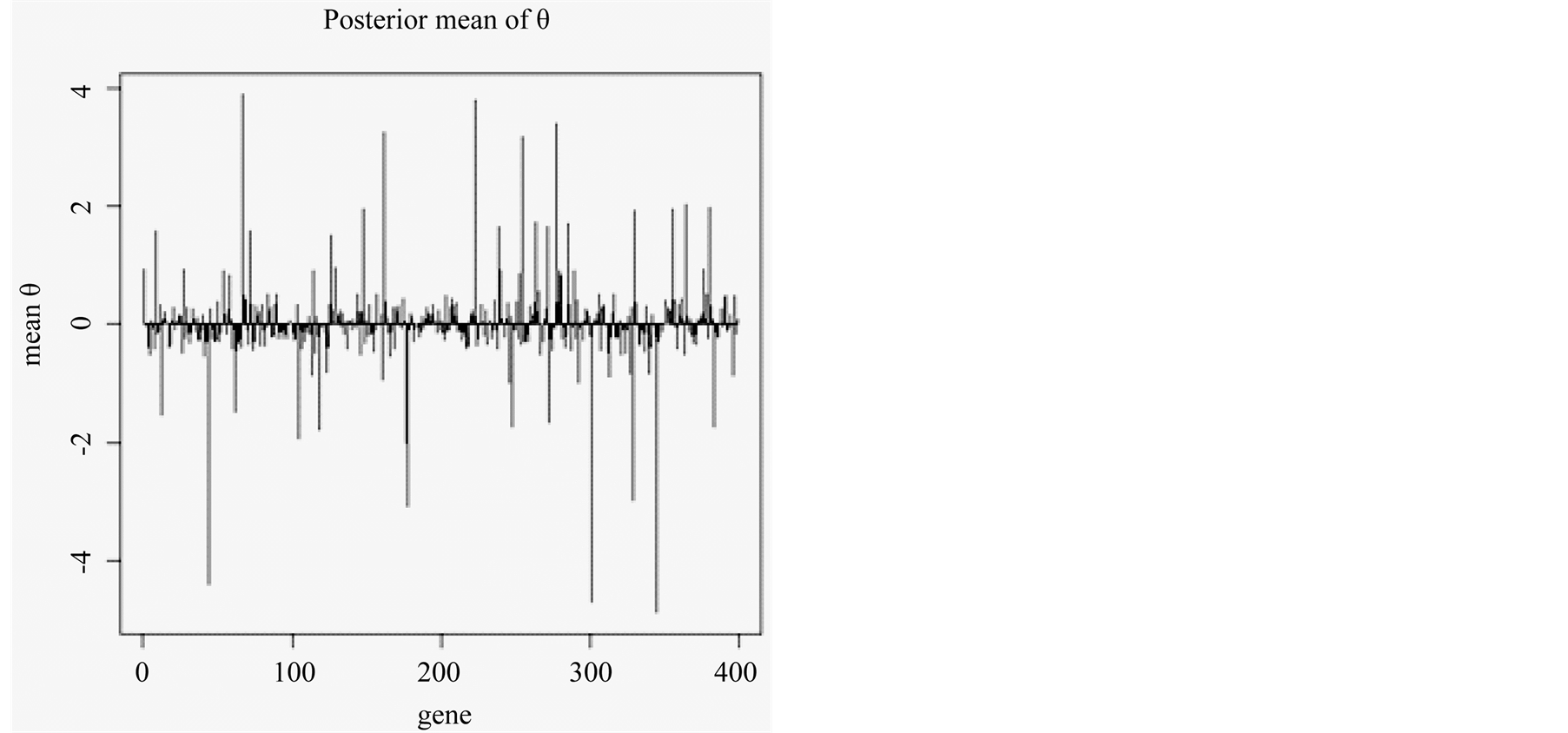
Figure 1. Posterior mean of qs associated with gene 1 to gene 398.

Table 1. Overall average accuracy of SBGLM, SVM and Random Forest using 10 and 50 marker genes.
Table 2. Average classification accuracy of prostate cancer subtypes in the test group using SBGLM, SVM and Random Forrest with 10 and 50 marker genes.
better than Random Forrest at classifying Benign, PIN and MET. These results indicate that the performance of SBGLM is comparable to Random Forrest in classifying subtypes of prostate cancer, although the results for both methods are sensitive to the number of selected marker genes.
Since the results of SBGLM were comparable to Random Forrest, we next asked if SBGLM gene rankings were more or less relevant to the biological mechanisms associated with prostate cancer progression. As a first step in evaluating the biological relevance for the top ranked genes in the models, we used a literature based method called Geneset Cohesion Analysis Tool (GCAT) [3] . GCAT is a web-based tool that determines the functional coherence p-values of gene sets based on latent semantic analysis of Medline abstracts [3] . Table 3 shows the average GCAT literature derived p-values (LPv) for the top 100 genes obtained from 50 runs of SBGLM and Random Forrest as well as the top 100 genes based on the p-value rank ordering of single gene analysis using ordinal logistic regression. We found that on average, SBGLM produced more functionally cohesive gene list (LPv = 0.007) compared classical logistic regression (LPv = to 0.047) and Random Forest (LPv = 0.131). Notably, 96% of the runs had smaller LPv than 0.047, produced by linear regression p-value ranking. We next manually evaluated the functional association between the top ranked genes in each model with prostate cancer biology. For this comparison, the median run for each model was chosen. We found that 6 out of 10 genes ranked by SBGLM has some association with prostate cancer (data not shown), whereas only 3 out of the top 10 genes ranked by SVM and Random Forrest had associations with prostate cancer (data not shown). Based on these results, we conclude that although SBGLM produces comparable classification accuracy as Random Forrest, it identifies more biologically relevant gene markers.
5. Discussion
Complex diseases and biological processes are caused by interaction of multiple genes (gene products). Hence, current approaches which rely on single variable analysis have limited utility in understanding molecular mechanisms and identification of genetic biomarkers for classification of diseases [5] [21] -[23] . Moreover, most genomic approaches collect data for a much larger set of gene variables compared to the number of samples being investigated. Therefore, highly regularized approaches, such as penalized regression models, are needed to identify non-zero coefficients, enhance model predictability and avoid over-fitting [28] . Lastly, continuous response variables which are a requirement of linear regression methods are not applicable to response variables (phenotypes) that are dichotomous or polytomous. To address these limitations, we developed a sparse Bayesian multinomial model and evaluated its performance using prostate cancer gene expression data. We found that the SBGLM classification accuracy of prostate cancer subtypes were comparable to Random Forrest. However, SBGLM identified more biologically relevant gene sets (Table 3). Based on these results, we posit that SBGLM may be a better approach to simultaneously identify marker genes for classifications as well as gaining insights into the molecular mechanisms of the phenotype under investigation. Interestingly, using fewer genes, SBGLM had very good discrimination performance for classifying benign (99.6% accuracy) versus metastatic prostate cancer (95.4% accuracy), but the model discrimination was weaker for PIN and PCA (Table 2). These results are consistent with the previous observation that PIN and PCA share markedly similar expression signatures [2] . We found that increasing the number of marker genes to 50 does not improve discrimination between PIN and PCA, suggesting that different molecular mechanisms may underlie the progression of PIN to PCA.
Random Forests are an ensemble method for classification that has been shown to have good performance in many bioinformatic applications. However, Random Forrest is prone to over-fitting in datasets with noisy classification tasks. In addition, it is very hard to interpret the classifications made by Random Forests. Furthermore, if data contain categorical variables with different number of levels, Random Forest favors variables with more levels, making the variable importance measures unreliable [38] .
It is important to note that the classification accuracy of all three models were compared using a selected set of 398 genes which were obtained based on p-value of single gene analysis using an ordinal regression model. Hence, this biases the initial gene selection process. It is possible that some biologically relevant genes to the prostate cancer progression might have been missed by this analysis due to low signal. One way to perform an initial gene selection could be to consider gene pathway information as described previously by others [39] . Our
Table 3 . Literature based functional cohesion p-values (LPv) of the top 100 genes obtained from three different models.
future plan is to evaluate SBGLM performance using pathway driven feature selection methods while considering more complex variance-covariance matrix structure which takes into account gene-gene interactions. Also, future work will investigate using different link functions and their effects on the model performance. Lastly, we plan to extend the model to other sparse models which use specialized prior distributions with heavier tails that might offer more robustness properties.
References
- Park, T. and Casella, G. (2008) The Bayesian lasso. Journal of the American Statistical Association, 103, 681-686. http://dx.doi.org/10.1198/016214508000000337
- Tomlins, S.A., Mehra, R., et al. (2007) Integrative Molecular Concept Modeling of Prostate Cancer Progression. Nature Genetics, 39, 41-51. http://dx.doi.org/10.1038/ng1935
- Xu, L., Furlotte, N., Lin, Y., Heinrich, K., Berry, M.W., George, E.O. and Homayouni, R. (2011) Functional Cohesion of Gene Sets Determined by Latent Semantic Indexing of PubMed Abstracts. PLoS ONE, 6, Article ID: e18851.
- Cao, J. and Zhang, S. (2010) Measuring Statistical Significance for Full Bayesian Methods in Microarray Analyses. Bayesian Analysis, 5, 413-427. http://dx.doi.org/10.1214/10-BA608
- Devore, J. and Peck, R. (1997) Statistics: The Exploration and Analysis of Data. Duxbury Press, Pacific Grove.
- Thomas, J.G., Olson, J.M., Tapscott, S.J. and Zhao, L.P. (2001) An Efficient and Robust Statistical Modeling Approach to Discover Differentially Expressed Genes Using Genomic Expression Profiles. Genome Research, 11, 1227-1236. http://dx.doi.org/10.1101/gr.165101
- Pan, W. (1996) A Comparative Review of Statistical Methods for Discovering Differentially Expressed Genes in Replicated Microarray Experiments. Bioinformatics, 18, 546-554. http://dx.doi.org/10.1093/bioinformatics/18.4.546
- Dudoit S., Fridlyand, J. and Speed, T.P. (2002) Comparison of Discrimination Methods for the Classification of Tumors Using Gene Expression Data. Journal of the American Statistical Association, 97, 77-87. http://dx.doi.org/10.1198/016214502753479248
- Troyanskaya, O.G., Garber, M.E., Brown, P., Botstein, D. and Altman, R.B. (2002) Nonparametric Methods for Identifying Differentially Expressed Genes in Microarray Data. Bioinformatics, 18, 1454-1461. http://dx.doi.org/10.1093/bioinformatics/18.11.1454
- Bae, K. and Mallick, B.K. (2004) Gene Selection Using a Two-Level Hierarchical Bayesian Model. Bioinformatics, 20, 3423-3430. http://dx.doi.org/10.1093/bioinformatics/bth419
- Logsdon, B.A., Hoffman, G.E. and Mezey, J.G. (2010) A Variational Bayes Algorithm for Fast and Accurate Multiple Locus Genome-Wide Association Analysis. BMC Bioinformatics, 11, 58. http://dx.doi.org/10.1186/1471-2105-11-58
- Wu, T.T., Chen, Y.F., Hastie, T., Sobel, E. and Lange, K. (2009) Genome-Wide Association Analysis by Lasso Penalized Logistic Regression. Bioinformatics, 25, 714-721. http://dx.doi.org/10.1093/bioinformatics/btp041
- Yang, J., Benyamin, B., McEvoy, B.P., Gordon, S., Henders, A.K., Nyholt, D.R., Madden, P.A., Heath, A.C., Martin, N.G., Montgomery, G.W., Goddard, M.E. and Visscher, P.M. (2010) Common SNPs Explain a Large Proportion of the Heritability for Human Height. Nature Genetics, 42, 565-569. http://dx.doi.org/10.1038/ng.608
- Tibshirani, R. (1996) Regression Shrinkage and Selection via the Lasso. Journal of the Royal Statistical Society, 58, 267-288.
- Li, J.H., Das, K., Fu, G.F., Li, R.Z. and Wu, R.L. (2011) The Bayesian Lasso for Genome-Wide Association Studies. Bioinformatics, 27, 516-523. http://dx.doi.org/10.1093/bioinformatics/btq688
- Zou, H. (2006) The Adaptive Lasso and Its Oracle Properties. Journal of the American Statistical Association, 101, 1418-1429. http://dx.doi.org/10.1198/016214506000000735
- Nott, D.J. and Leng, C. (2010) Bayesian Projection Approaches to Variable Selection in Generalized Linear Models. Computational Statistics & Data Analysis, 54, 3227-3241. http://dx.doi.org/10.1016/j.csda.2010.01.036
- Yi, N. and Xu, S. (2008) Bayesian LASSO for Quantitative Loci Mapping. Genetics, 179, 1045-1055.http://dx.doi.org/10.1534/genetics.107.085589
- Fan, J. and Li, R. (2001) Variable Selection via Nonconcave Penalized Likelihoodand Its Oracle Properties. Journal of the American Statistical Association, 96, 1348-1360. http://dx.doi.org/10.1198/016214501753382273
- Ye, J.P., Li, T., Xiong, T. and Janardan, R. (2004) Using Uncorrelated Discriminant Analysis for Tissue Classification with Gene Expression Data. IEEE/ACM Transactions on Computational Biology and Bioinformatics (TCBB), 1, 181-190.
- Calvo, A., Xiao, N., Kang, J., Best, C.J., Leiva, I., Emmert-Buck, M.R., Jorcyk, C. and Green, J.E. (2002) Alterations in Gene Expression Profiles during Prostate Cancer Progression: Functional Correlations to Tumorigenicity and DownRegulation of Selenoprotein-P in Mouse and Human Tumors. Cancer Research, 62, 5325-5335.
- Dalgin, G.S., Alexe, G., Scanfeld, D., Tamayo, P., Mesirov, J.P., Ganesan, S., DeLisi, C. and Bhanot, G. (2007) Portraits of Breast Cancer Progression. BMC Bioinformatics, 8, 291. http://dx.doi.org/10.1186/1471-2105-8-291
- Pyon, Y.S. and Li, J. (2009) Identifying Gene Signatures from Cancer Progression Data Using Ordinal Analysis. BIBM ‘09. IEEE International Conference on Bioinformatics and Biomedicine, Washington DC, 1-4 November 2009, 136-141.
- Hans, C. (2009) Bayesian Lasso Regression. Biometrika, 96, 835-845. http://dx.doi.org/10.1093/biomet/asp047
- Nelder, J. and Wedderburn, R. (1972) Generalized Linear Models. Journal of the Royal Statistical Society, 135, 370-384. http://dx.doi.org/10.2307/2344614
- McCullagh, P. and Nelder, J. (1989) Generalized Linear Models. Chapman and Hall, London.
- Madsen, H. and Thyregod, P. (2011) Introduction to General and Generalized Linear Models. Chapman & Hall/CRC, London.
- Pike, M.C., Hill, A.P. and Smith, P.G. (1980) Bias and Efficiency in Logistic Analysis of Stratified Case-Control Studies. International Journal of Epidemiology, 9, 89-95.
- Knight, K. and Fu, W. (2000) Asymptotics for Lasso-Type Estimators. The Annals of Statistics, 28, 1356-1378. http://dx.doi.org/10.1214/aos/1015957397
- Xu, H., Caramanis, C. and Mannor, S. (2010) Robust Regression and Lasso. IEEE Transactions on Information Theory, 56, 3561-3574. http://dx.doi.org/10.1109/TIT.2010.2048503
- Gilks, W., Richardson, S. and Spiegelhalter, D. (1996) Markov Chain Monte Carlo in Practice. Chapman and Hall, London.
- Gelfand, A. and Smith, A.F.M. (1990) Sampling-Based Approaches to Calculating Marginal Densities. Journal of the American Statistical Association, 85, 398-409. http://dx.doi.org/10.1080/01621459.1990.10476213
- Albert, J. and Chib, S. (1993) Bayesian Analysis of Binary and Polychotomous Response Data. Journal of the American Statistical Association, 88, 669-679. http://dx.doi.org/10.1080/01621459.1993.10476321
- Benjamini, Y. and Hochberg, Y. (1995) Controlling the False Discovery Rate: A Practical and Powerful Approach to Multiple Testing. Journal of the Royal Statistical Society. Series B, 57, 289-300.
- Karatzoglou, A., Smola, A., Hornik, K. and Zeileis, A. (2004) kernlab—An S4 Package for Kernel Methods in R. Journal of Statistical Software, 11, 1-20. http://www.jstatsoft.org/v11/i09/
- Liaw, A. and Wiener, M. (2002) Classification and Regression by Random Forest. R News, 2, 18-22.
- Breiman, L. (2001) Random Forests. Machine Learning, 45, 5-32. http://dx.doi.org/10.1023/A:1010933404324
- Boulesteix, A.L., Janitza, S., Kruppa, J. and König, I.R. (2012) Overview of Random Forest Methodology and Practical Guidance with Emphasis on Computational Biology and Bioinformatics. Wiley Interdisciplinary Reviews: Data Mining and Knowledge Discovery, 2, 493-507. http://dx.doi.org/10.1002/widm.1072
- Subramanian, A., Tamayo, P., Mootha, V.K., Mukherjee, S., Ebert, B.L., Gillette, M.A., Paulovich, A., Pomeroy, S.L., Golub, T.R., Lander, E.S. and Mesirov, J.P. (2005) Gene Set Enrichment Analysis: A Knowledge-Based Approach for Interpreting Genome-Wide Expression Profiles. Proceedings of the National Academy of Sciences of the United States of America, 102, 15545-15550. http://dx.doi.org/10.1073/pnas.0506580102