Open Journal of Statistics
Vol.2 No.5(2012), Article ID:25365,6 pages DOI:10.4236/ojs.2012.25061
Tree Model Optimization Criterion without Using Prediction Error
National Agriculture and Food Research Organization, Agricultural Research Center,
Graduate School of Life and Environmental Sciences, University of Tsukuba, Tsukuba, Japan
Email: nonpara@gmail.com
Received September 20, 2012; revised October 30, 2012; accepted November 6, 2012
Keywords: Cross-Validation; Model Optimization Criterion; One-SE Rule; Significance Level; Tree Model
ABSTRACT
The use of prediction error to optimize the number of splitting rules in a tree model does not control the probability of the emergence of splitting rules with a predictor that has no functional relationship with the target variable. To solve this problem, a new optimization method is proposed. Using this method, the probability that the predictors used in splitting rules in the optimized tree model have no functional relationships with the target variable is confined to less than 0.05. It is fairly convincing that the tree model given by the new method represents knowledge contained in the data.
1. Introduction
In constructing a tree model (e.g., Breiman et al. [1], Takezawa [2], Chapter 9 of Chambers and Hastie [3]), the optimization of the number of decision rules is crucial; it is equivalent to the selection of predictors in multiple regression and to the optimization of smoothing parameters in nonparametric regression. 10-fold crossvalidation is a well-known technique among diverse methods of optimizing the number of decision rules. 10-fold cross-validation partitions the sample into 10 groups at random. Then, nine groups are used as the training data for creating a model and the remaining group is used as the validation data for estimating the predictive error of the model. This procedure is repeated several times and the predictive errors are averaged; it yields a reliable predictive error. Minimization of the prediction error leads to the optimal value of the cost complexity measure (hereafter, it is called![]() ). The optimal value of
). The optimal value of ![]() gives the optimal number of decision rules.
gives the optimal number of decision rules.
However, experience with real data shows that the number of decision rules optimized by 10-fold crossvalidation tends to be slightly larger than the optimal one in terms of prediction error. Thus, the One-SE rule(e.g., p. 78 in Breiman et al. [1])is widely used to derive a number of decision rules somewhat smaller than that given by 10-fold cross-validation. The One-SE rule employs the smallest number of decision rules in the range of the standard error of the number of decision rules optimized by 10-fold cross-validation. Although this method is based on an intuitive idea that, since the number of decision rules yielded by 10-fold cross-validation is too large, the reduction in the number should be permitted in the range of the standard error of the number of decision rules; the large number of real examples of tree models demonstrate the efficacy of this method.
On the other hand, a tree model is widely applied as a tool for extracting beneficial knowledge from multidimensional data. That is, the use of a tree model is a typical method of data mining. This is because it is presumed that each decision rule in a tree model summarizes information contained in data in simple form. However, the contents of a tree model optimized solely by 10-fold cross-validation or 10-fold cross-validation using the One-SE rule are not always regarded as a series of knowledge given by data because a tree model produced with the intention to reduce prediction error may contain erroneous knowledge. Optimization methods centering on prediction error do not consider this possibility explicitly at least. Since a tree model is derived using a finite number of data sets, the possibility that erroneous knowledge is contained in a tree model cannot be 0. However, if we can estimate this possibility, we can quantify the usefulness of a tree model from a point of view different from that of prediction error.
In this paper, we present a method of optimizing a tree model using the possibility that the model contains apparently inappropriate decision rules; the method does not utilize prediction error. It is an application of the method of selecting predictors that almost certainly have linear relationships with the target variable in multiple regression (Takezawa [4]). In the subsequent section, we show using real data that the relationship between the prediction error of a tree model and the appropriateness of decision rules is not simple. We therefore suggest a method of optimizing the number of decision rules using the probability that a tree model contains inappropriate decision rules in the following section. In the end, a numerical simulation of this method and the application of this method to the analysis of the real data are shown.
2. Definition of the Problem Using Real Data
We employ the first 200 sets of “HousePrices” data contained in the R package “AER”. The data consisting of 12 variables is about the sale prices of houses sold in the city of Windsor, Canada in 1987. Applicants for the predictors ( ) and the target variable (y), listed below, are selected from the 12 variables. These predictors and target variables are the same as those adopted in the multiple linear regression on p. 68 in Verbeek [5].
x1: Logarithmically transformed lot size of a property in square feet.
x2: Number of bedrooms.
x3: Number of full bathrooms.
x4: Is there central air conditioning? (“Yes” = 1, “No” = 0)
y: Logarithmically transformed sale price of a house.
R package “mvpart” (version 1.6-0) was used to produce tree models using this data. By assigning “xv = ‘min’” and “xvmult = 50” in the command “mvpart()”, which is contained in the mvpart package, 10-fold crossvalidation is carried out 50 times to obtain ![]() which yields a minimal prediction error. Using the resultant
which yields a minimal prediction error. Using the resultant![]() the tree model (Figure 1) is constructed. This tree model is composed of 10 decision rules. Such a tree model is equivalent to a partition of feature space of by recursive binary partitions using decision rules; refer to Figure on Figure 9.2 on page 268 in Hastie et al. [6] and Figure 8.3 on page 398 in Duda [7]. Since x1 stands for the size of a house, y should increase when x1 is large. However, the third decision rule from the left shows that y is smaller when x1 is larger than or equal to 8.175 when compared with a smaller x1. On the other hand, when “xv = ‘1se’” is set instead of “xv = ‘min’”,
the tree model (Figure 1) is constructed. This tree model is composed of 10 decision rules. Such a tree model is equivalent to a partition of feature space of by recursive binary partitions using decision rules; refer to Figure on Figure 9.2 on page 268 in Hastie et al. [6] and Figure 8.3 on page 398 in Duda [7]. Since x1 stands for the size of a house, y should increase when x1 is large. However, the third decision rule from the left shows that y is smaller when x1 is larger than or equal to 8.175 when compared with a smaller x1. On the other hand, when “xv = ‘1se’” is set instead of “xv = ‘min’”, ![]() obtained by 10-fold cross-validation using the One-SE rule results in the tree model shown in Figure 2. It consists of two decision rules. The tree model produced by a naive 10-fold cross-validation is considerably different from that produced by 10-fold cross-validation using the One-SE rule.
obtained by 10-fold cross-validation using the One-SE rule results in the tree model shown in Figure 2. It consists of two decision rules. The tree model produced by a naive 10-fold cross-validation is considerably different from that produced by 10-fold cross-validation using the One-SE rule.
Next, the fifth predictor (x5), which takes random values, is added and simulation is carried out. When the values of x5 are unrelated to y and a tree model is produced, for the tree model to be appropriate, it should have no decision rules with x5; it is a necessary condition.
Firstly, a uniform random number that takes values between 0 and 1 is used as x5. Simulation with this x5 was conducted 500 times while varying the initial value of each pseudo-random number. Then, when a naive 10- fold cross-validation is used, the tree models produced contain decision rules with x5 in 143 simulations. Since some tree models contain plural decision rules with x5, the total number of decision rules with x5 appearing in 143 simulations is 261. When 10-fold cross-validation using the One-SE rule is adopted, the number of tree models containing decision rules with x5 is 2, and the total number of decision rules with x5 in the two tree models is 4.
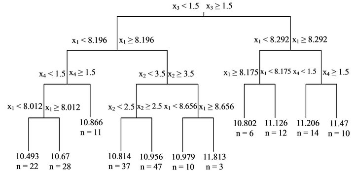
Figure 1. Tree model produced by the first 200 sets of “HousePrices” data. A set of values of predictors is put at the top of the model and goes down following the decision rules to reach the terminal node where the estimate of the target value is shown. “n=” at the terminal node indicates the number of data sets arriving at the terminal node. α is optimized by 10-fold cross-validation.
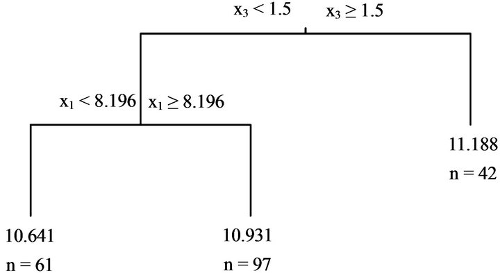
Figure 2. Tree model produced by the first 200 sets of “HousePrices” data. “n=” indicates the number of data sets arriving at the terminal node. α is optimized by 10-fold cross-validation using the One-SE rule.
Next, x5 is set at either 0 or 5 and the probabilities of taking both values are equal. This simulation is repeated 500 times while varying the initial value of each pseudorandom number. When a naive 10-fold cross-validation is used, 90 simulations resulted in tree models containing decision rules with x5. The total number of decision rules with x5 in those tree models is 105. When 10-fold crossvalidation using the One-SE rule is used, only one tree model contains a decision rule with x5; the total number of decision rules with x5 is 1.
The above simulations indicate that when![]() is optimized using prediction error given by 10-fold crossvalidation to produce a tree model and some of the predictors are not related to the target variable, the probability of constructing decision rules with a predictor not associated with the target variable is not constant. This probability depends on the characteristics of the predictor that has no relationship with the target variable. Hence, when a tree model is constructed using real data by 10-fold cross-validation, it is difficult to determine the probability that a predictor used in a decision rule in the tree model is not associated with the target variable. Furthermore, if 10-fold cross-validation using the OneSE rule is adopted, this probability is reduced markedly. This tendency, however, may prevent the construction of beneficial decision rules.
is optimized using prediction error given by 10-fold crossvalidation to produce a tree model and some of the predictors are not related to the target variable, the probability of constructing decision rules with a predictor not associated with the target variable is not constant. This probability depends on the characteristics of the predictor that has no relationship with the target variable. Hence, when a tree model is constructed using real data by 10-fold cross-validation, it is difficult to determine the probability that a predictor used in a decision rule in the tree model is not associated with the target variable. Furthermore, if 10-fold cross-validation using the OneSE rule is adopted, this probability is reduced markedly. This tendency, however, may prevent the construction of beneficial decision rules.
The simulations thus far show that a naive 10-fold cross-validation and 10-fold cross-validation using the One-SE rule do not ensure probability that a tree model contains decision rules with an inappropriate predictor. Therefore, when we aim to obtain decision rules that give sound knowledge, optimization methods based on prediction error are not appropriate. We need a method that controls the probability of obtaining meaningless decision rules.
3. A New Method of Optimizing a Tree Model
To control the probability of producing meaningless decision rules in a tree model, we suggest a method of investigating a tree model yielded using data in which the data of some predictors are unrelated to the target variable. That is, when the data of predictors are represented as 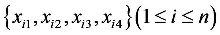 (n is the number of data) and the data of the target variable are represented as
![]() , we carry out the procedure below to optimize
, we carry out the procedure below to optimize ![]() to be used in the construction of a tree model.
to be used in the construction of a tree model.
1) n data are sampled at random with replacement from . The sample is named
 .
.
2) n data are sampled at random with replacement from . The sample is named
 .
.
3) n data are sampled at random with replacement from . The sample is named
 .
.
4) n data are sampled at random with replacement from . The sample is named
 .
.
5) m values ( ) are prepared as applicants for
![]() .
.
6) Using one value in , a tree mode is produced using eight predictors and
![]() . Since the values of
. Since the values of  depend on the initial value of the random numbers, 500 data sets are produced while varying the initial value of the pseudo random number, and a tree model for each data set is constructed.
7) Tree models that have no decision rules with  are chosen from 500 tree models and such tree models are counted for each
 . The number of such tree models is denoted gj.
8) The procedures from (1) to (7) using each  result in
 . The value closest to 475 is selected from
 .
.  corresponding to the chosen gj is denoted
![]() .
.
9) Using![]() , a tree model is produced using
, a tree model is produced using .
.
The adoption of a decision rule with a predictor not related to the target variable is equivalent to the rejection of the null hypothesis in the test of simple regression; the null hypothesis states that the gradient is 0 despite the values of the predictor being random and not related to the target variable. Hence,  yielded using this algorithm is called the risk rate. In this example, when the risk rate given by
 is roughly 0.05,
  is denoted
![]() . Then, the probability that a tree model contains decision rules with a predictor that has no functional relationship with the target variable is less than 0.05.
. Then, the probability that a tree model contains decision rules with a predictor that has no functional relationship with the target variable is less than 0.05.
The condition that the probability of using a random predictor in a tree model is less than 0.05 is a necessary condition for constructing a tree model that represents a series of knowledge contained in the data. However, other necessary conditions along this line are possible. For example, if the data of all predictors are replaced with data given by bootstrapping the data of respective predictors, the resultant tree model should have no decision rules. Hence, the probability of obtaining a tree model with one or more decision rules should be small. Then, making this probability less than 0.05 will be a necessary condition for constructing a tree model for the purpose of knowledge acquisition. However, if all predictors are random, we determine whether a decision rule should be set for each predictor, and no decision rule is created if we conclude that a decision rule cannot be constructed for all predictors. On the other hand, the algorithm suggested above considers the possibility of obtaining decision rules with either one of x5, x6, x7, or x8 beyond the decision rules with x1, x2, x3, and x4 as well as the decision rule with either one of x5, x6, x7, or x8 as the first decision rule. Therefore, the Algorithms (1)-(9) described above give stricter conditions than the algorithm performed by making all predictors random.
4. Numerical Simulation
The simulation data consists of four data sets of predictors  and one data set of the target variable
are all uniform random numbers between 0 and 1. ![]() are obtained using
are obtained using
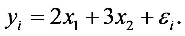 (1)
(1)
![]() are realizations of
are realizations of  (a normal distribution with 0 mean and 0.52 variance). Therefore,
  and
and  have no functional relationships with the target variable.
400 sets of the simulation data were produced. Tree models are constructed using the method suggested in the previous section. Ten tree models contain decision rules with x3 but not those with x4, and four tree models contain decision rules with x4 but not those with x3. No tree models contain decision rules with x3 and those with x4. That is, the probability that tree models contain decision rules with a random predictor is less than 0.05.
In this simulation, tree models are constructed using eight predictors of which six, i.e., from x3 through x8, are uniform random numbers between 0 and 1. Then, since the probability that a tree model contains decision rules with one of the four variables from x5 through x8 is roughly 0.05, we can infer that the probability that a tree model contains decision rules with either x3 or x4 is roughly 0.025. In fact, the number of random predictors with the same statistical characteristics is not necessarily exactly proportional to the probability that a tree model contains decision rules with those predictors because a decision rule with x3, for example, is constructed beyond that with x5; this means that a decision rule with x3 is not constructed if that with x5 does not exist. However, the probability that a decision rule with a random predictor is constructed beyond another decision rule with another random predictor is considered to be small. Hence, let us assume that four predictors are uniform random numbers between 0 and 1, and that the probability that a tree model contains decision rules with those predictors is controlled to be 0.05. Then, if two predictors are uniform random numbers between 0 and 1, the probability that a tree model contains decision rules with one of the two predictors will be about 0.025.
Next, the same simulation with a risk rate of 0.2 instead of 0.05 is carried out. As a result, 31 tree models contain decision rules with x3 but not those with x4. On the other hand, 28 tree models contain decision rules with x4 but not those with x3. One tree model contains decision rules with x3 and those with x4. That is, the probability that a tree model contains decision rules with a random predictor is less than 0.2.
This time, both  and
and  are replaced with a random variable that takes 0 with a 0.5 probability and 5 with a 0.5 probability. Using this data, the same simulation is carried out. The result is that two tree models contain decision rules with x3 but not those with x4, and one tree model contains decision rules with x4 but not those with x3. No tree models contain decision rules with x3 and those with x4. Although the probability of obtaining decision rules with a random predictor is changed by changing the characteristics of
  and
and , the probability remains less than 0.05.
Then, risk rate was shifted from 0.05 to 0.2, and the same simulation was carried out. Eight tree models contain decision rules with x3 but not those with x4, and four tree models contain decision rules with x4 but do not contain those with x3. No tree models contain decision rules with x3 and those with x4. This simulation also shows that the probability that a tree model contains decision rules with a random predictor is less than 0.2.
All of the above simulations indicate that, using the method suggested in the previous section, if some of the predictors are random, the probability that a tree model contains a decision rule with one of those predictors falls below the assigned risk rate. Therefore, we find that when some of the predictors of data are not associated with the target variable, the probability that a tree model contains decision rules with one of those predictors is controlled to be less than the risk rate defined in the previous section.
5. Real Data Example
The method suggested in Section 3 was applied to the analysis of the real data treated in Section 2. For this purpose, ![]() is fixed at one of the 21 values of
is fixed at one of the 21 values of
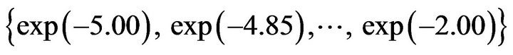 . The values of the predictors from
  through
  were generated by bootstrapping the values from
  through
 , respectively. The simulation using these data yielded the results shown in Table 1. This table shows the number of tree models that contain no decision rules with a random predictor when a value is given as
  and when the data of predictors from x5 through x8 are random. Since 500 simulations with respective conditions are conducted, 500 given by −2.00 as
 , for example, indicates that none of the tree models obtained contain decision rules with one of the predictors from x5 through x8.
Table 1 shows that the risk rate given by −3.2 as  is
is , which is close to 0.05. Hence, the risk rate of the tree model given by this condition is 0.05. The resultant tree model is shown in Figure 3. This tree model consists of four decision rules. Meanwhile, since the risk rate yielded using −3.65 as
  is
is , which is close to 0.2. The tree model given by this condition is shown in Figure 4. This tree model is composed of six decision rules. The decision rules in these two tree models are reasonable. They are better than that shown in Figure 1 in this regard.
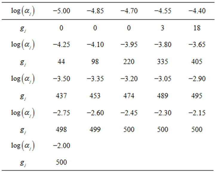
Table 1. Number of tree models that contain no decision rules with a random predictor.
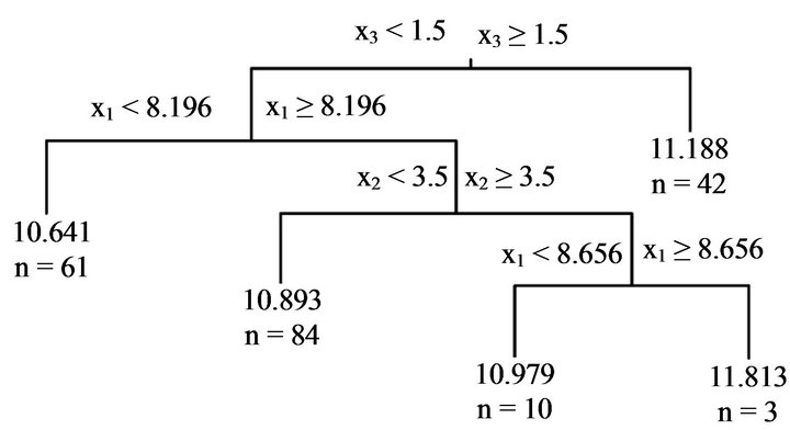
Figure 3. Tree model obtained using the first 200 sets of “HousePrices” data. Risk rate is set at 0.05.
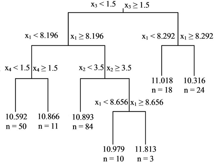
Figure 4. Tree model obtained using the first 200 sets of “HousePrices” data. Risk rate is set at 0.2.
However, although the procedure that produced the tree models shown in Figures 3 and 4 satisfies the necessary conditions for a method of constructing a tree model, it may not satisfy sufficient conditions. Even if a satisfactory tree model construction method has to satisfy other conditions, it does not result in a tree model that has a larger number of decision rules than the tree model shown in Figure 3 or Figure 4. In this respect, the tree model shown in Figure 1 does not satisfy the necessary conditions that a tree model for knowledge acquisition has to satisfy.
6. Conclusions
In conventional modelling methods, rules and the functional relationships contained in a model constructed by a model selection method based on prediction error are viewed to be a series of knowledge extracted from data. The background of this philosophy is instrumentalism. That is, if an obtained model has superior ability in terms of prediction, the rules and functional relationships contained in it (i.e., knowledge used in the model) are considered dependable. This appears to be an appropriate product of the pragmatic methodology of data analysis. However, if the probability that some of the rules or functional relationships contained in a model that is useful in terms of prediction are generated only by accident is not negligible, we cannot consider that a tree model optimized on the basis of prediction error represents unequivocal knowledge. Therefore, prediction error should not be used in modelling for the purpose of knowledge acquisition. Instead, a tree model, for example, should be optimized by controlling the probability that inappropriate rules or functional relationships are obtained.
Decision rules in a tree model are often considered to instinctively represent a series of knowledge existing in the data. Hence, if some decision rules contradict the findings on the phenomenon that generates the data, the overall reliability of the tree model may be questioned. However, if a tree model is optimized by 10-fold crossvalidation, there is no assurance regarding the probability that the tree model contains meaningless decision rules. Hence, such a tree model should not be regarded as an extract of knowledge. Meanwhile, when 10-fold crossvalidation using the One-SE rule is used, the number of decision rules becomes considerably smaller than obtained using a naive 10-fold cross-validation. This means that the probability of obtaining meaningless decision rules is small. This probability, however, cannot be estimated. Hence, we cannot determine whether the resultant tree model is appropriate for knowledge acquisition. That is, we cannot quell doubts that the number of decision rules in a tree model is unduly small and that the required decision rules are lacking.
On the other hand, the method suggested here does not use the concept of prediction error given by 10-fold cross-validation or related procedures. When we consider that the term “data mining” was coined by comparing data analysis to mineral extraction, this new method studies the efficacy of a mining method by replacing part of the data with a true nonmineral. This method, however, makes us question whether attention to decision rules with apparently unneeded decision rules is sufficiently effective for obtaining an appropriate tree model. We thus should optimize a tree model by considering how decision rules with a nonrandom predictor are constructed. The concept of the power of test as well as risk rate should be discussed. Prediction error should be taken into account to a certain degree.
In the above sense, there is room for further examination of our suggested method. We, however, were successful in showing a new point of view on the construction of a tree model, which is completely different from those based on prediction error. Although conventional regression analysis has been developed in the fields of statistical test and prediction, this new method suggests that a third field of knowledge discovery should be added to the existing two fields. We hope that we can further develop research on a new modeling methodology that yields models for acquiring knowledge or for obtaining persuasive rules and functional relationships.
REFERENCES
- L. Breiman, F. Friedman, C. J. Stone and R. A. Olshen, “Classification and Regression Trees,” Chapman and Hall/CRC, London, 1984.
- K. Takezawa, “Introduction to Nonparametric Regression,” Wiley, Hoboken, 2006.
- J. M. Chambers and T. J. Hastie, “Statistical Models in S,” Chapman and Hall/CRC, London 1991.
- K. Takezawa, “Flexible Model Selection Criterion for Multiple Regression,” Open Journal of Statistics, Vol. 2, No. 4, 2012, pp. 401-407.
- M. Verbeek, “A Guide to Modern Econometrics,” 2nd Edition, Wiley, Hoboken, 2004.
- T. Hastie, R. Tibshirani and J. Friedman. “Elements of Statistical Learning,” 1st Edition, Springer, New York, 2001.
- R. O. Duda, P. E. Hart and D. G. Stork, “Pattern Classification,” 2nd Edition, Wiley-Interscience, Hoboken, 2000.