Open Journal of Statistics
Vol.1 No.2(2011), Article ID:5855,16 pages DOI:10.4236/ojs.2011.12007
Small Sample Estimation in Dynamic Panel Data Models: A Simulation Study
School of Statistics, University of the Philippines Diliman, Quezon City, Philippines
E-mail: lorelie.santos@gmail.com, ernielb@yahoo.com
Received March 17, 2011; revised April 2, 2011; accepted April 10, 2011
Keywords: Dynamic Panel Data Model, Within-Groups Estimator, First-Difference Generalized Method of Moments Estimator, Parametric Bootstrap
Abstract
We used simulated data to investigate both the small and large sample properties of the within-groups (WG) estimator and the first difference generalized method of moments (FD-GMM) estimator of a dynamic panel data (DPD) model. The magnitude of WG and FD-GMM estimates are almost the same for square panels. WG estimator performs best for long panels such as those with time dimension as large as 50. The advantage of FD-GMM estimator however, is observed on panels that are long and wide, say with time dimension at least 25 and cross-section dimension size of at least 30. For small-sized panels, the two methods failed since their optimality was established in the context of asymptotic theory. We developed parametric bootstrap versions of WG and FD-GMM estimators. Simulation study indicates the advantages of the bootstrap methods under small sample cases on the assumption that variances of the individual effects and the disturbances are of similar magnitude. The boostrapped WG and FD-GMM estimators are optimal for small samples.
1. Introduction
Panel data combine cross-sectional and time series information. Since the temporal dependencies for each unit could vary significantly, a dynamic parameter is desirable to relax the parametric constraints into the model. Dynamic panel data (DPD) model postulates the lagged dependent variable as an explanatory variable. Just like in univariate time series analysis, modeling the dependency of the time series on its past value(s) gives valuable insights on the temporal behavior of the series. [1] noted that many economic relationships are dynamic in nature and the panel data allow the researcher to better understand the dynamics of structural adjustment exhibited by the data.
A good number of dynamic panel data estimators have been proposed and thoroughly characterized in the literature. The within-group (WG) estimator, among the early estimation method for DPD, provides consistent estimate for static models. In DPD models, [2] showed that the WG estimator of the coefficient of the lagged dependent variable parameter is downward biased and the bias only disappears as the number of time units grows larger. Thus, the WG estimator is known to be biased whenever the time-dimension  is fixed, even if the cross-section dimension
  is large.
The inconsistency of the WG estimator leads to the development of DPD coefficient parameter estimators that are consistent for large  and fixed or large
 , e.g., the use of instrumental variables (IV). For the IV estimators, [3] used either the dependent variable lagged two periods or its first-differences as instruments. Even the development of the generalized method of moments (GMM) estimators for DPD coefficient parameters is based on the IV approach. [4] proposed GMM estimator that uses all available lags at each period as instruments for the equations in first differences, this is now known as the first-difference generalized method of moments estimator (FD-GMM). [5] proposed the level GMM estimator which is based on the level of the model and uses lagged difference variables as instruments. [6] further proposed the now called system GMM estimator which uses both the lags of the level and first difference as instruments.
The DPD model estimators have exhibited good asymptotic properties, see for example [2], [7], and [8]. Some work investigated the small sample properties of the said estimators, e.g., [9] and [10]. There are numerous studies on the properties of dynamic panel data model but are mostly focusing on data sets with large cross-section and small time dimensions. Other studies highlight datasets with sizeable cross-section dimensions and moderately-sized time dimensions.
We used intensive simulations to investigate both the small and large sample properties of two of the simplest and oldest DPD estimators, the within-groups and first-difference generalized method of moments estimators of the AR(1) DPD model. We also propose the use of parametric bootstrap procedure in the WG and FD-GMM for the boundary scenario, i.e., when asymptotic optimality of WG and FD-GMM fail.
As [11] pointed out, the application of bootstrap methodology in panel data analysis is currently in its embryonic stage. The bootstrap estimators proposed in this study can answer the possible limitations of the estimators by [8]. Over a short period, it is common for processes over time to be easily affected by random shocks. Thus, if long period data are used, it is very likely that structural change will manifest and the modeler will either incorporate the change into the model (more complicated), or analyze the series by shorter periods, leading to small sample data where the proposed estimator is applicable.
2. Dynamic Panel Data Model
Suppose the dynamic behavior of a time series for unit i (yit) is characterized by the presence of a lagged dependent variable among the regressors, i.e.
 (1)
(1)
where  is a constant,
  is
is  vector of explanatory/exogenous variables, and
  is
is  vector of regression coefficients.
  follows a two-way error component model
  where
where  and
and  are the (unobserved) individual and time specific effects which are assumed to stay constant for given
  over
over  and for a given
  over
over , respectively; and
  represents the unobserved random shocks over
  and
and . The unobserved individual-specific and/or time-specific effects
  and
and , are assumed to follow either the fixed effects model (FE) or the random effects model (RE). If Equation (1) assumes a RE model and if
  follow a one-way error component model
 , then the individual and time specific effects are
  and
and  independent of each other and among themselves. When
  and
and  are treated as fixed constants, the usual assumptions are
  and
and . [12], [1] and [13] give detailed discussions on dynamic panel data models.
Consider the following AR(1) dynamic panel data model without exogenous variable
 (2)
(2)
where  is the dependent variable,
  is the regression coefficient (parameter of interest) with
 ,
,  is the unobserved heterogeneity or individual effect which has mean 0 and variance
  and
and  is unobserved disturbance with mean 0 and variance
 . To facilitate the computations of estimators of model 2, let
 ;
; ’;
’; ’;
’; ’; and
 ’ (a
’ (a  vector of ones). Equation (2) can be written as
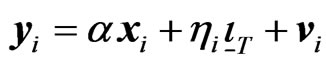 (3)
(3)
[8] considered several estimators of , e.g., the within group/covariance (WG) estimator (also called fixed effects (FE) estimator), covariance (CV) estimator (or least squares dummy variable (LSDV) estimator), and the first-difference generalized method of moments (FD-GMM) estimator (one-step level GMM estimator proposed by [4]). In the computation of
  and
and  further notations are used:
[8] defined the WG estimator as
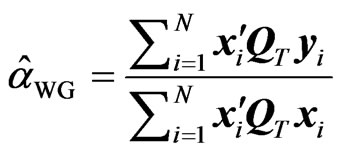 (4)
(4)
where ,
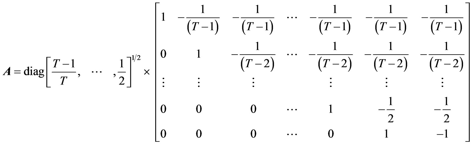
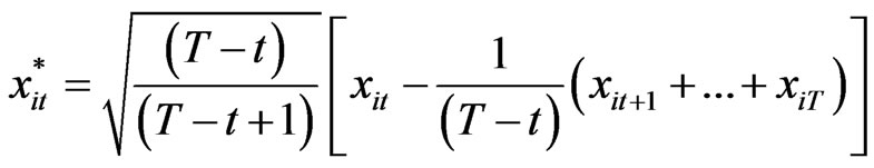
,  is called the WG operator of order T. WG estimator may also be written in terms of the forward orthogonal deviations operator
 , an upper triangular-like matrix, with dimension
  and with the following characteristics:
 ,
,  and
and . Let
. Let  and
and , then WG estimator is given by
 (5)
(5)
[8] further analyzed an asymptotically efficient FD-GMM estimator given by
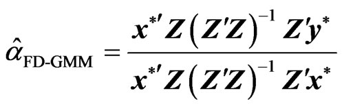 (6)
(6)
where . A computationally useful alternative expression for
  is:
is:
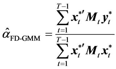 (7)
(7)
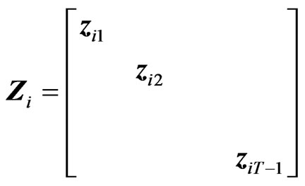
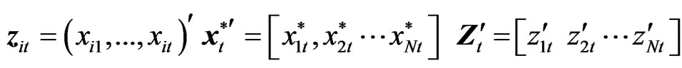
where  and
and  are the
  vectors whose ith elements are
  and
and , respectively,
  and
and  is the
  matrix whose ith row is
 . As pointed by [8],
  is nonsingular when
 , but the projections involved remain well defined in any case. Without loss of generality, the condition
  was maintained because the FD-GMM estimator is motivated in a situation where T is smaller than N and it is straightforward to extend the results in their paper to allow for any combination of values of T and N by considering a generalized formulation of 7 using
 , where
  is the Moore-Penrose inverse of
 . In this way,
 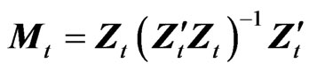 if
if  and
and  if
if . Thus, the contribution of terms with
  to the FDGMM formula coincide with the corresponding terms for WG.
[8] derived the asymptotic properties of several dynamic panel data estimators namely, within groups (WG), first-difference generalized method of moments (FD-GMM), limited information maximum likelihood (LIML), crude GMM and random effects ML estimators of the AR(1) parameter of a simple DPD model with random effects.
As observed by [8],  is consistent for
 , regardless of
 . However, as
 , the asymptotic distribution of
  may contain an asymptotic bias term, depending on the relative rates of increase of
  and
and . When
 , the asymptotic variance of WG estimator is the same as the of GMM estimator and they have similar (negative) asymptotic biases in which for WG has order
 . On the other hand,
  is a consistent estimator for
  as both
  and
and , provided that
 . Also, the number of the FD-GMM orthogonality conditions
  tends to infinity as
 . The F
  is asymptotically normal, provided that
  and
and . When
 , the asymptotic variance of FDGMM estimator is the same as the WG estimator and they have similar expression for their (negative) asymptotic biases in which for FD-GMM has order
 . When
 , the asymptotic bias of GMM is smaller than the bias of WG. When
 , the two asymptotic biases are equal and when
 , the asymptotic bias in the WG estimator disappears.
From a simulation study, [7] observed that the variance of the WG estimators is usually much smaller than the variance of consistent GMM estimators, see [2], [7-9], [14], and [8] for further details.
3. The Bootstrap Method
The bootstrap is a useful tool for estimation in finite samples. Bootstrap procedure entails the estimation of parameters in a model through resampling with a large number of replications, [15]. [16] developed the idea of bootstrap procedure known as a nonparametric method of resampling with replacement and it stems from older resampling methods such as the jackknife method and delta method. Originally, the bootstrap requires independent observations, i.e.,  consisting of
  observations
 ,
,  , …,
, …,  , a random sample from the true distribution
  generating the data. The data generates the empirical distribution
 , a discrete distribution that assigns equal probability to the
  observations of the observed sample, hence,
 . The bth bootstrap sample is a vector
  consisting of
  observations
 ,
,  , …,
, …,  (
( ), obtained by sampling with replacement B times from the empirical distribution
 . In each of the
  bootstrap samples, the estimator of a parameter in a particular model is computed, resulting to
 ,
,  , …,
, …,  , where
  is an estimator of a parameter, say θ.
For time series models, the sieve bootstrap and the block bootstrap are recently introduced. The sieve bootstrap starts by fitting the most adequate model and the behavior of the empirical distribution of the residuals is analyzed. The bootstrap errors  are generated by resampling
  times from the empirical distribution
 ,
, . In order to generate the bth bootstrap sample
 , each element of
  is determined by the recursion
 , where the starting values for
  are set to zero and the first
  generated values are thrown away, so that the needed bth bootstrap sample
  is obtained.
On the other hand, the block bootstrap resamples from overlapping blocks of consecutive observations to generate the bootstrap replicates, see [17] and [15] for a more comprehensive discussion of bootstrap methods for time series models.
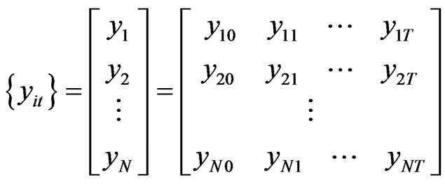
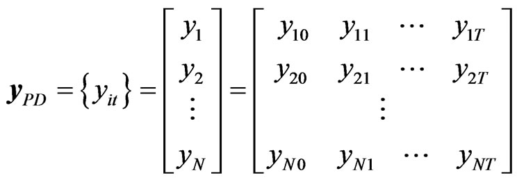
To define the bootstrap for dynamic panel data models, suppose  is defined as measurements from different cross-section units of the population over different time periods, so that the data can be represented by
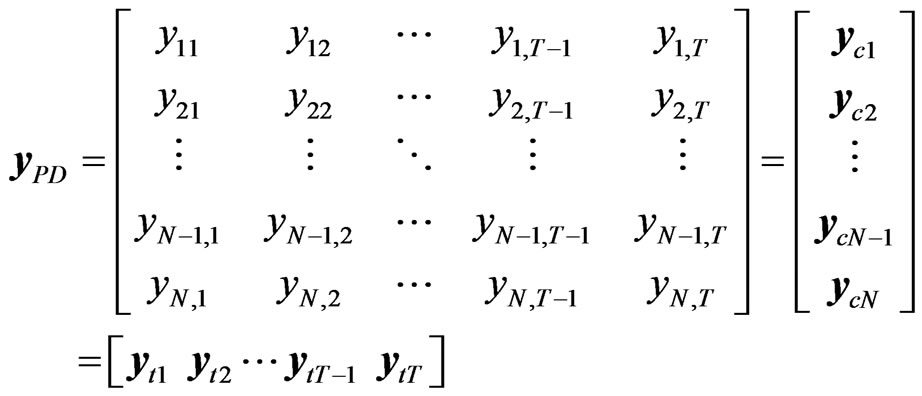 (8)
(8)
The bth bootstrap sample is the  matrix
 , given by
 (9)
(9)
 is generated by doing the AR-sieve bootstrap procedure for panel data. [11] identified five bootstrap methodologies for panel data namely: i.i.d. bootstrap, individual bootstrap, temporal bootstrap, block bootstrap and double resampling bootstrap. The i.i.d bootstrap refers to the bootstrap procedure defined by [16]. Each of the
  elements of the observed data matrix
  is given
  probability in the empirical distribution
 . The elements of the bth bootstrap sample
  in (9) are obtained by resampling with replacement from the empirical distribution
 .
.
The rows of  in (8) are resampled with replacement in order to determine the bth bootstrap sample
  of the form in (9) in the individual bootstrap procedure. On the other hand, in the temporal bootstrap procedure, the columns of
  in (8) are resampled with replacement in order to create the bth bootstrap sample
  of the form (9). The resampling procedure for the block bootstrap is in the temporal dimension, so that the data matrix of the form (8) is used. The difference between the block bootstrap and the temporal bootstrap is on the sampling of blocks of columns of
  in (8) instead of single column/period in the temporal bootstrap case. Let
 , where
  is the length of a block and thus, there are
  non-overlapping blocks. Block bootstrap resampling entails the construction of
  such as (9) with columns obtained by resampling with replacement the
  non-overlapping blocks columns of
  in (8).
Given the data matrix , double resampling is a procedure that constructs the bth bootstrap sample
  by resampling columns and rows of
 . Two schemes can be chosen, the first is a combination of individual and temporal bootstrap and the second is a combination of individual and block bootstrap. Therefore, as the name of this bootstrap procedure implies, it involves two/double stages. The first stage is to construct an intermediate bootstrap sample
  by performing individual bootstrap. The second stage uses the intermediate bootstrap sample
  as a matrix where either temporal bootstrap or block bootstrap is applied to produce the bth bootstrap sample
 .
.
4. Bootstrap Procedure for Dynamic Panel Data Estimators
While the literature clearly illustrates the asymptotic optimality of WG and FD-GMM estimators, there are doubts on their performance under small samples. Many panel data are usually formed from small samples of time points and/or panel units because of the structural change or random shocks that may occur in bigger/larger datasets. For small samples, we propose to use parametric bootstrap on WG and FD-GMM in mitigating the bias and inconsistency that these estimators are known to exhibit for small samples.
We consider the AR(1) dynamic panel data model:
 (10)
(10)
where  is the parameter,
  is the individual effect with mean zero and variance
 , and disturbances
  with mean zero and variance
 . The bootstrap procedure below uses AR Sieve in replication, steps follow:
Step 1: Given  generated from the model in 10, we have
  time-series data
 (11)
(11)
For each cross-section unit , we assume an AR(1) model with slope
  and intercept
 , i.e.,
 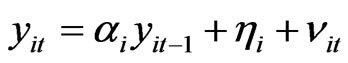 ,
, . Using the method of least squares we obtain the estimators
  and
and  for the parameters.
Step 2: Compute , the average of all
 ’s over all cross-section units, i.e.,
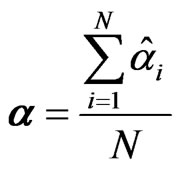 .
.
Step 3: For a fixed cross-section unit , the predicted values
 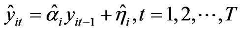 is computed and used to compute the MSE=
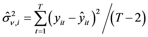 .
.
Simulate  sets of
  from
from .
.
Step 4: Reconstruct the panel data  using
using  in step 2,
  in step 1 and one of the
  sets of
  in step 3. The reconstructed panel data
  is obtained using equation (10), i.e.,
  ,
,  , where
  comes from
 , the ith element of the first column of matrix 11.
Step 5: Do step 4 B times, taking note that the used set of  should not be used again in subsequent reconstruction of the panel data. There will result to
  panel data
 .
.
Step 6: Compute WG and FD-GMM estimators using Equations (5) and (7) respectively, for each of the  panel data sets.
Step 7: Resample the  WG and FD-GMM estimates in step 6.
When sample size is small, there is a tendency for estimators based on asymptotic optimality to become erratic. The AR sieve is used to reconstruct as many time series as possible that capture the same structure as the original data. Resampling from each of the recreated data and computation of WG and FD-GMM for each resamples can alleviate instability caused by small samples, inheriting the optimal properties of the bootstrap methods.
5. Simulation Study
In the simulation study, we used AR(1) with individual random effects model given in Equation (10), i.e.,  ,
, . We used a Monte Carlo design that aims to examine both the asymptotic and finite (small) sample properties of the two estimators of the parameter α. Where the asymptotic properties are examined, the cross-section dimension go as large as 500 (see [18]) or as small as 50 (see [8]). We consider
  corresponding to the large cross-section dimension scenario. On the other hand,
  is the largest time dimension used in studies about asymptotic properties (see [8]). Some studies use smaller
  values such as
  and
and  along with
  and
and  to show the asymptotic properties of estimators, especially the GMM type, see [8]. We assume large time dimension with
 . When smaller
  is used such as,
  and
and  (see [10], [19]), even
  is as large as 100, it still exhibit small sample properties of the estimator, specifically the GMM estimator. We consider as small time dimensions cases with
  and
and . If the objective is to examine the finite sample properties of estimators especially the WG estimator, small to moderate sizes for both the cross-section and time dimensions are commonly used, e.g.,
 ;
;  and
and ;
; ;
; ;
; , for details, see [9].
There are few studies where the time series and crosssection dimensions are both small such, e.g.,  , T = 10, 20, see [7]. Small cross-section dimensions considered are
  and
and , and moderate cross-section dimensions are
  and
and . We also consider as moderate time dimension cases where
  and
and . Therefore, the values for
  and
and  can capture the settings for both short and wide panel, typical of a micro-panel and long and narrow panel, which is a common set-up for macro-panels.
In panel data, the observations in a particular crosssection unit comprise a time series. Since, we employ a dynamic panel data model, the AR(1) coefficient parameter , can be viewed as the common slope parameter for the
  time series in an
  panel data. Thus, given a time series with
  observations, our choice of the values of the AR(1) coefficient parameter
  ranges from an almost white noise series, where
  is very small, e.g., when
  to an almost unit root series where
  is very near to one, that is, when
 .
.
The values for the variance of the individual effects accounts for both fixed effects when  and random effects, that is,
 . The variance of the random disturbance is set at
 . Table 1 presents the different combination of parameter values for a total of 625 parameter combinations.
First, we assume values of the ratio of the individual effects variance to the random disturbance variance, the possible values of the cross-section unit and time unit sizes that are considered small samples and varying values of the slope parameter. Then we generate N sets of 10,000 ’s where
  and we generate N
  ’s where
 , by choosing one value for the variance ratio
  from Table 1. The generated
 ’s and the individual effect for the ith cross-section
  is used to compute the initial value
  for each cross-section unit
 , using Equation (10), the initial value is
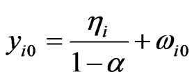 , where
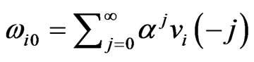 .
.
Also, we generate 
 ’s where
 . Then a value for
  is chosen from Table 1 and using the N
 ’s and
 ’s, a set of dynamic panel data
 ,
, ;
;  can be generated from Equation (10), i.e.,
 . This will give rise to a data matrix of the form 11,
The analysis for the asymptotic and finite sample properties of the WG and FD-GMM estimators was done using 100 replications, in this case, 100 panel data sets  for each of the 625 designs/parameter combinations. The WG and FD-GMM estimates for a total of 62,500 data sets using Equations 5 and 7 respectively. The mean, median, quartiles of WG and FD-GMM estimate for each of the 625 sets containing 100 replicates of data are computed.
We compare the performance of the two estimators  and
and  using the sample medians and interquartile ranges. Note that the two estimators are both downward biased, so that comparisons will be more meaningful if resistant measures are used to assess the bias and efficiency. Hence, in assessing the finite sample properties of the two estimators, the median bias and median percent bias are used. On the other hand, efficiency is examined by looking at the dispersion using a more resistant measure like the interquartile range as compared to the standard deviation.
If we denote the WG and FD-GMM estimates from the  th replicate by
  and
and , we get
 ,
,  ,…,
,…,  and
and ,
,  ,…,
,…,  respectively. Denote the sorted values of
  by
by  and
and  by
by . The sample median for a particular design is
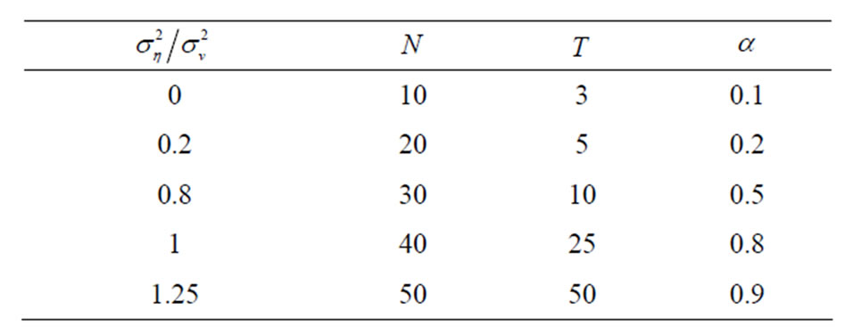
Table 1. Monte carlo designs.
given by  =
= for the WG estimator and
 =
= for the FD-GMM estimator. The interquartile range for WG estimator is
  and the corresponding interquartile range for the FDGMM estimator is equal to
  .
.
[8] computed the asymptotic approximations to the bias given by  and
and  for WG and FD-GMM estimators, respectively.
6. Results and Discussion
We report the Monte Carlo simulations on the WG and FD-GMM estimators for various combinations of values of  and
and , and relatively wide range of values for
  and
and . The main focus of the analysis is on the bias of the WG and FD-GMM estimators as the number of cross-section dimension
  and the number of time dimension
  changes. The change in bias as the true value of the coefficient parameter
  varies is also shown. The effect of the variance ratio between the individual effect and the random disturbance on the bias of the two estimators is explored.
6.1. Effect of the Sample Size on the Bias
The marginal effect of varying the cross-section dimension  and the time dimension
  are presented separately. The joint effect of
  and
and  is also presented as [8] emphasized that the asymptotic bias of the DPD estimators depend on the relative rates of increase of
  and
and .
.
In theory, the cross-section dimension  has no effect on the bias of the WG estimator. This is confirmed in the simulation exercise, where the bias of WG estimator is relatively constant as
  varies, given that
  is fixed. On the other hand, the theory is that the FD-GMM estimator has a bias of order
 , that is, the bias decreases as
  becomes large. This pattern is not perfectly observed in the simulation. For instance, when the variance ratio
 , only 10 out of the 25 cases have shown the pattern of decreasing bias of the FD-GMM estimates as the number of cross-section dimension increases. Also, when the variance ratio
 , only 10 out of the 25 cases have shown the pattern of decrease in bias as
  increases. A summary of the range of values of bias as percentage of the true parameter value for the FD-GMM estimator focusing on varying the cross-section dimension
  is presented in Table 2. For a moderate time dimension
 , we could expect a FD-GMM estimate with a bias from 14% to 47% for
 , from 8% to 39% for
  and from 6% to 38% of the true value of the coefficient even when
 .
.
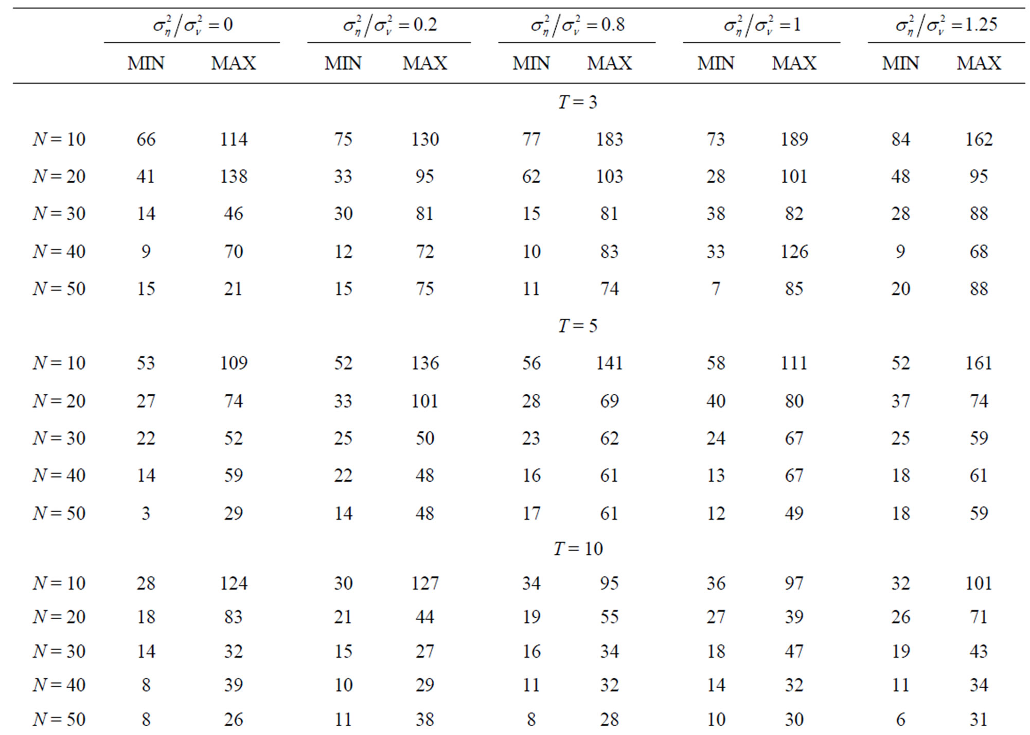
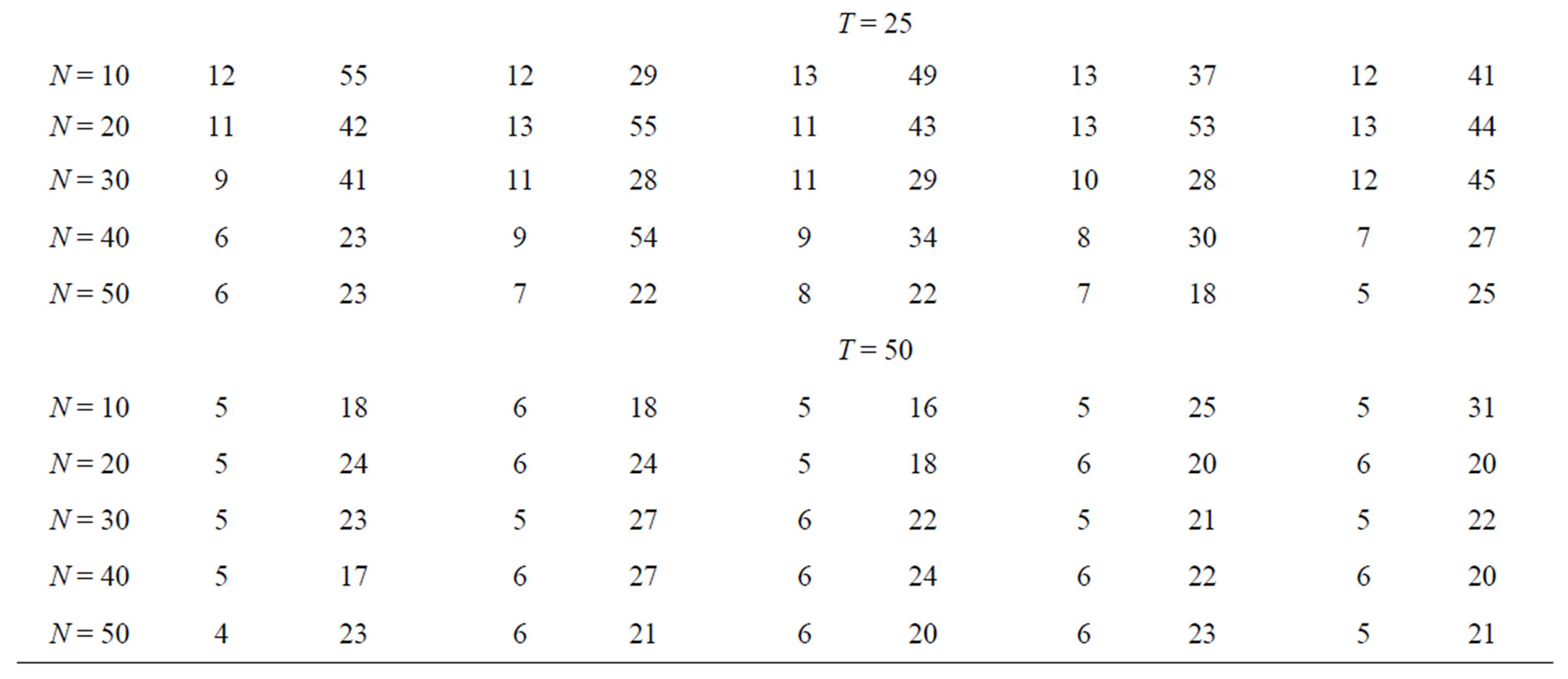
Table 2. Percent bias of .
.
The time dimension  affects the bias of the WG estimator. The WG estimator has bias of order
 , that is, as
  becomes larger, the WG bias becomes smaller. This is also observed in the simulation. As expected, as
  increases from 3 to 50, the bias reduces tremendously within acceptable levels as T is nearing 50. This pattern is implied by the increase of the magnitude of the medi-ans as
  becomes larger.
The FD-GMM estimator is known to be affected by the cross-section dimension , and the order of bias is
  and does not involve
 . [8] noted that consistency of the FD-GMM estimator requires
  where
where  and
and . This means that the bias of the FD-GMM estimator does not depend on
  alone but also
 . The FD-GMM estimates in the simulation exercise illustrate the decrease in bias as the time dimension increases, most specially for
 . Also, from Table 2, a FD-GMM estimate is within 6% to 127% of the true value, when
 , within 6% to 55% of the true value when
  and within 4% to 27% of the true value of the coefficient, implying the magnitude of FD-GMM bias decreases as
  increases.
A summary of the range of values of bias as percentage of the true parameter value for the WG estimator with varying time dimension  is presented in Table 3. For a small cross-section dimension
 , one could expect a WG estimate with a bias from 27% to 132% for
 , from 10% to 54% for
  and from 5% to 28% of the true value of the coefficient when
 . Even for large cross-section dimension, say
 , the WG estimates have similar range of percent bias as those estimate when
 . This indeed shows that there is notable decrease in the bias of WG estimates as
  increases whatever the value of
 .
.
Table 3. Percent bias of .
.
It is interesting to note that the relationship between bias and the sample size represented by the pair (N,T) also takes into account the relative rates of increase of  with respect to
  for the WG estimator and
  with respect to
  for the FD-GMM estimators. When we have a square panel, that is when the sample size is either, (
 ,
, ) or (
 ,
, ), the WG estimates and GMM estimates are almost the same. The similarity of the WG estimates to the GMM estimates is also seen for an almost square panel, such as (
 ,
, ), (
), ( ,
, ), and N = 40, T = 50. This confirms the theory of [8] that the asymptotic bias of WG and FD-GMM are the same when
 , we confirmed here to be also true for moderate samples and even small samples. When
 , regardless of the size of
 , the value of WG estimates are similar to the value of FD-GMM estimates. This is attributed to the fact that in the previously stated scenario, the time-series dimension is always greater than or equal to the cross-section dimension, in this case the workable formula for FD-GMM whenever
  is almost identical to the WG formula.
6.2. Effect of Parameter Values on the Bias
The first-order DPD model considered in this study has three parameters, but we focused only on the coefficient of the lagged dependent variable ( ). The two other parameters are the variances of the one-way random effects error component, namely the variance of the individual effect
  and the variance of the random disturbance
 . Instead of analyzing the effect of
  and
and  separately, we focus on the variance ratio
 .
.
Both the WG and FD-GMM estimators are downward biased, that is, the estimates are smaller than the true value of the coefficient parameter . As shown by [2] for WG estimator, the bias decreases as
  increases. This is true for both the WG and FD-GMM estimators as illustrated in the study. Also, one may think that the percent bias will increase as we decrease the value of
 , since the smaller the value of the denominator the larger the fraction becomes. This is confirmed in the results of simulation, the FD-GMM bias decrease as
  increase provided that
  is large.
The exact distribution of WG estimator is said to be invariant to both the variance of the individual effect  and the variance of the random disturbance
 , while the distribution of the FD-GMM estimator is invariant only to the variance ratio
 , see [8]. In the simulation exercise, varying the variance ratio does not show sizeable changes on the bias, when the sample size
  and the value of the parameter coefficient
  are fixed.
6.3. Other Asymptotic and Finite Sample Properties of WG and FD-GMM Estimators
We compare the median of the estimators to the approximate bias values computed by [8]. Percent different between the computed bias and the approximate bias are reported in Table 4. The following asymptotic properties: (a) when , the asymptotic bias of GMM is smaller than the WG bias, (b) when
 , the expression for the two asymptotic biases are equal and (c) when
 , the asymptotic bias in the WG estimator disappears, derived by Alvarez and Arellano (2003) still hold for smaller samples considered in this study. The findings of [7] that the WG is more efficient than GMM is also supported by the simulation study. Since the bias of WG estimator does not depend on
 , the values are similar, that is, the number of WG estimates with percent difference values less than 5% is almost the same for different values of
 . On the other hand, percent difference of FD-GMM estimate increases with
 . The asymptotic approximation of [8] performs well for
 , since 72.8% of the MC medians of FD-GMM estimates are within 20% of the approximated value.
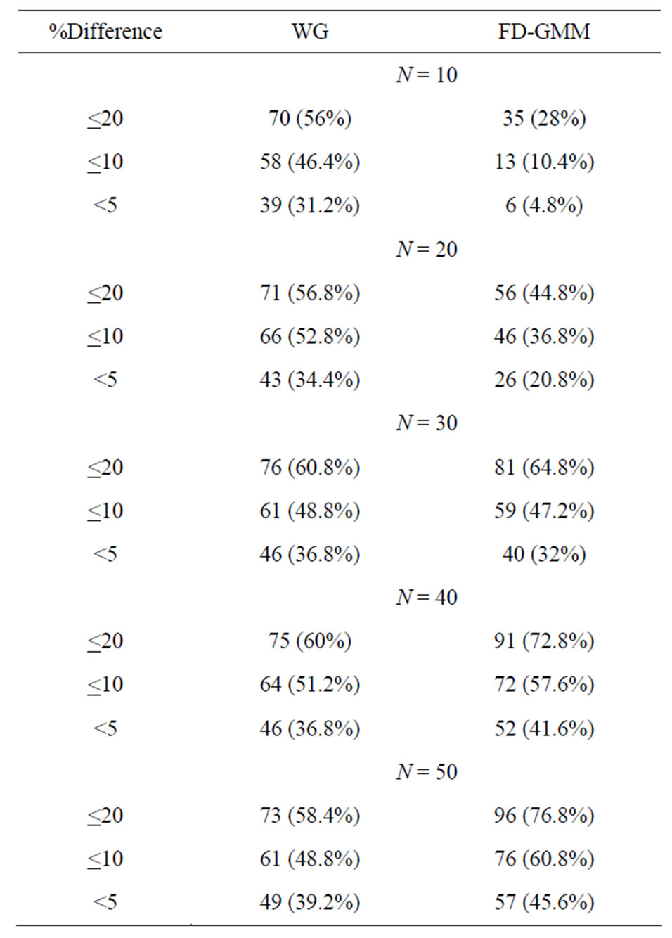
Table 4. Percent difference of bias estimates from asymptotic biases.
The bias of FD-GMM is smaller than the bias of WG estimates, that is 71 (56.8%) out of 125 cases follow this pattern. Note that 60% of the cases have the set-up , and the other 40% have the set-up
 . It is interesting to note that only when the variance of the individual effect
  equal to zero, we see that majority, that is, 20 out of the 25 cases considered have bias of FD-GMM less than the bias of WG. On the other hand, when
 , half of the cases have bias of FD-GMM smaller than bias of WG and the other half have bias of WG less than or equal to bias of FD-GMM. The cases where bias of WG is less than or equal to the bias of FD-GMM estimates have moderate to large
 , but when
 , the bias of WG is smaller and closer to the FD-GMM bias only when
  is at least 0.5. Specifically, bias of WG is close to bias of FD-GMM for square panels where
  and for
 .
.
We also analyzed moderately-sized cross-section dimension, i.e., . This allows for 80% of the 125 cases to have
  and the other 20% are designs where
 . We expect that more percentage of FDGMM estimates have smaller bias than WG estimates as compared to where the cross-dimension size is small. There are 90 (72%) of the 125 cases where bias of FD-GMM is smaller than the bias of WG. The other 35 (28%) cases have either large time-dimension, that is
  or larger value for the coefficient parameter, which is
 . This is intuitively true, since when
 ,
,  and the bias of WG is expected to be less than the bias of FD-GMM. For moderately-sized cross-section dimension, about 73% of the FD-GMM estimates have smaller bias than their WG counterpart and the other 27% have designs where the time dimension is large or the value of the coefficient of parameter is close to one.
Some 80% of the 125 cases have designs where T < N
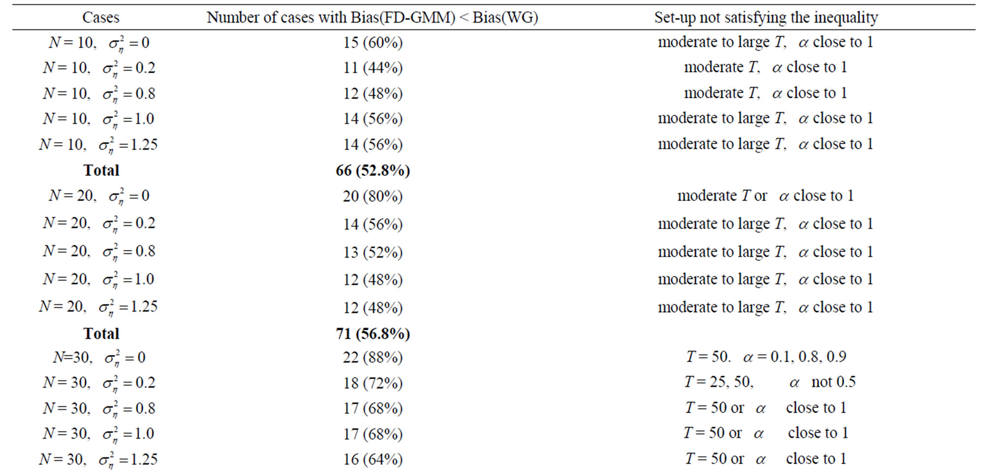
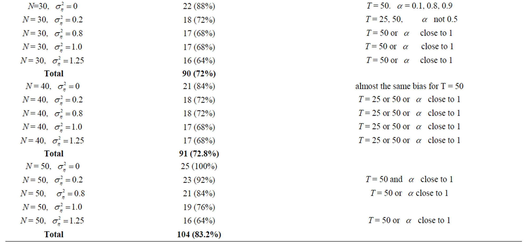
Table 5. Comparison of bias of WG and FD-GMM estimates.
and 20% of the cases come from square panel, that is,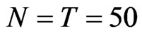 . We expect that most of the FD-GMM estimates have smaller bias than the WG estimates and when square panels are considered the biases are the same. There are 104 (83.2%) of the 125 cases considered has FD-GMM bias smaller than their WG counterpart. The other 21 (16.8%) cases have designs where the time dimension is large, that is,
  and the coefficient parameter is close to one, that is,
  0.8 or 0.9.
Table 6 summarizes comparison of the variability of WG and FD-GMM estimates as measured by the interquartile range (IQR). The WG estimates generally have less variability than FD-GMM estimates, for the mode-
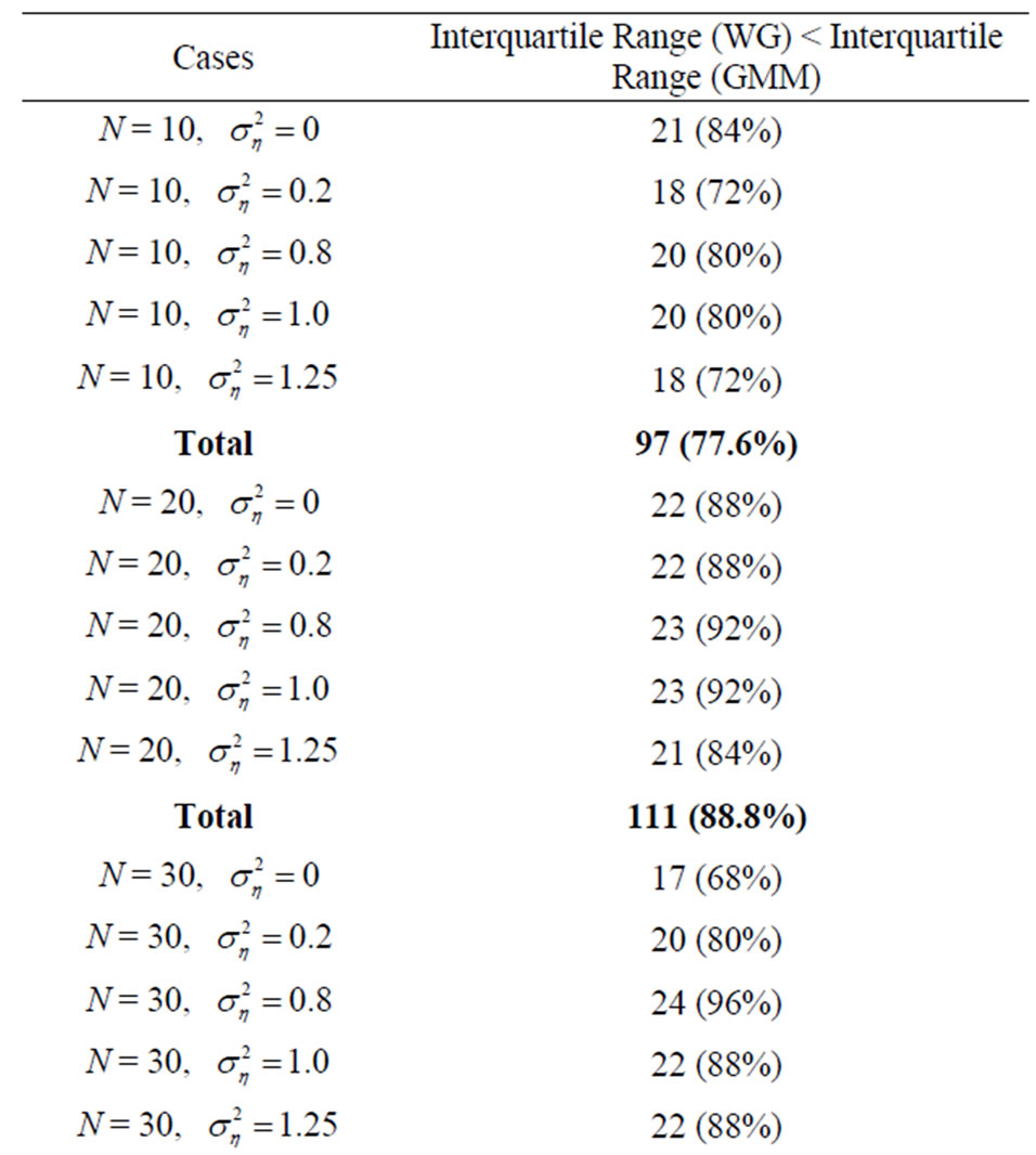
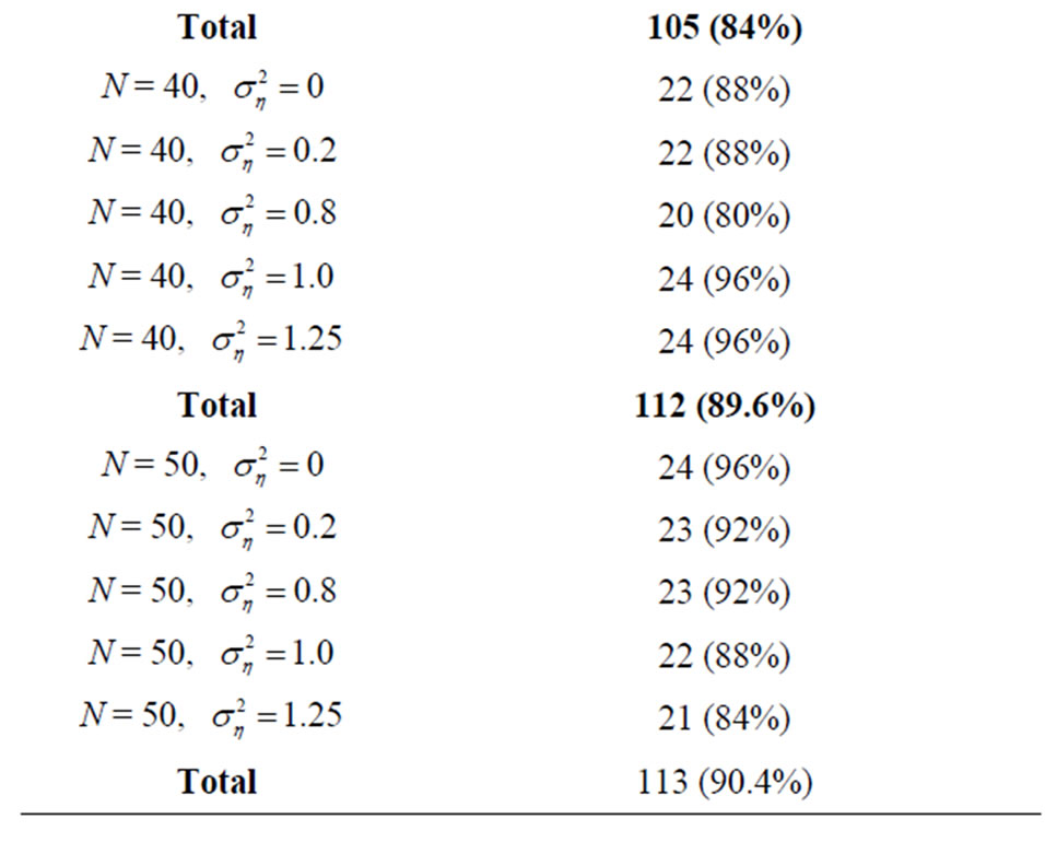
Table 6. Comparison of variability of WG and FD-GMM estimates.
rate size cross-section dimension. There are 105 (84%) cases where IQR of WG is less than IQR of FD-GMM. The strongest evidence that the WG estimator has smaller variability than FD-GMM is seen in the summary of Table 6, particularly, 113 (90.4%) of the 125 cases have IQR of WG smaller than IQR of FD-GMM.
6.4. Comparison of Bootstrapped DPD and Conventional DPD Estimators
To be able to assess the benefits from boostrapping the WG and GMM estimators, we identified settings in the simulation scenarios where they yield the largest bias. We report in Tables 7 and 8 the top 25 of estimates with the largest bias for both WG and GMM, together with their respective design specifications.
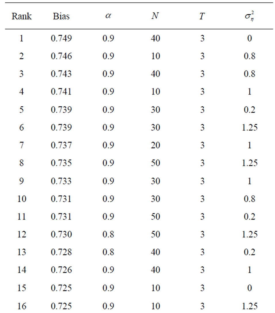
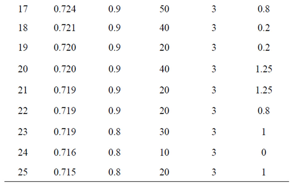
Table 7. 25 Largest bias of WG estimates and their design specifications.
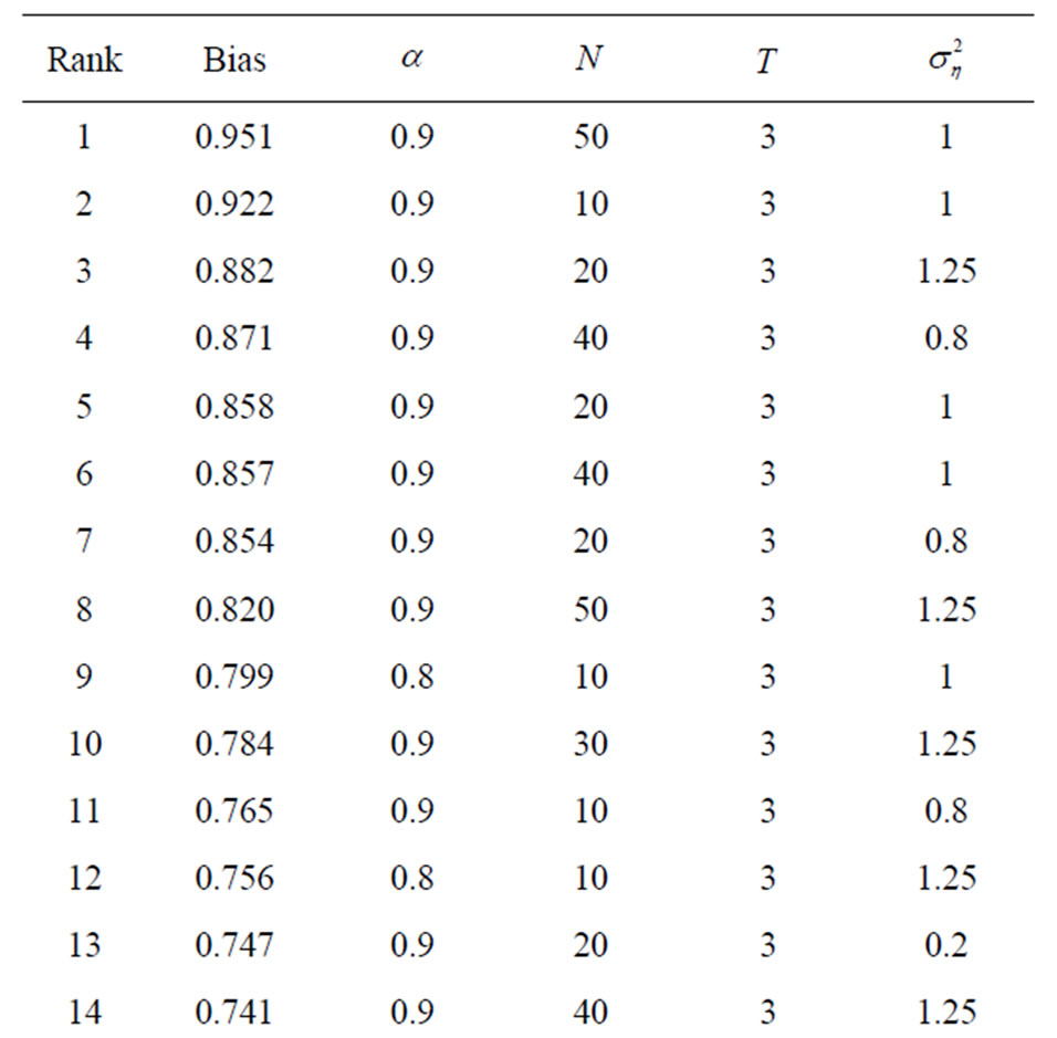
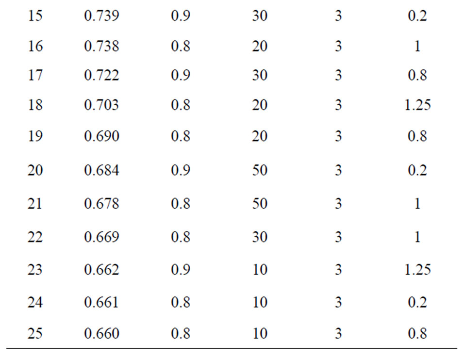
Table 8. 25 Largest bias of FD-GMM estimates and their design specifications.
The order of bias of the WG estimator is  and therefore, as
  increases the bias decreases. The order of bias of the GMM estimator is
  and thus, as
  increases, the bias decreases. In terms of the bias, the worst WG and GMM estimates came from designs with very small time dimension. This is congruent to the theoretical properties of the WG estimator, but at first quite surprising for GMM estimator. When
 , FD-GMM estimator uses only one instrument and thus equivalent to the IV estimator, less appealing than the GMM estimators. Moreover, the FD-GMM estimator when
 , does not show a decrease in bias as
  becomes larger.
It is known that the bias of WG estimator increases with the coefficient parameter , see [2] and [7]. In this simulation exercise, all the WG and GMM worst estimates came from designs with large
 , see Table 9. As the autoregression component of the model becomes nearly nonstationary, both WG and FD-GMM estimates can suffer tremendously.
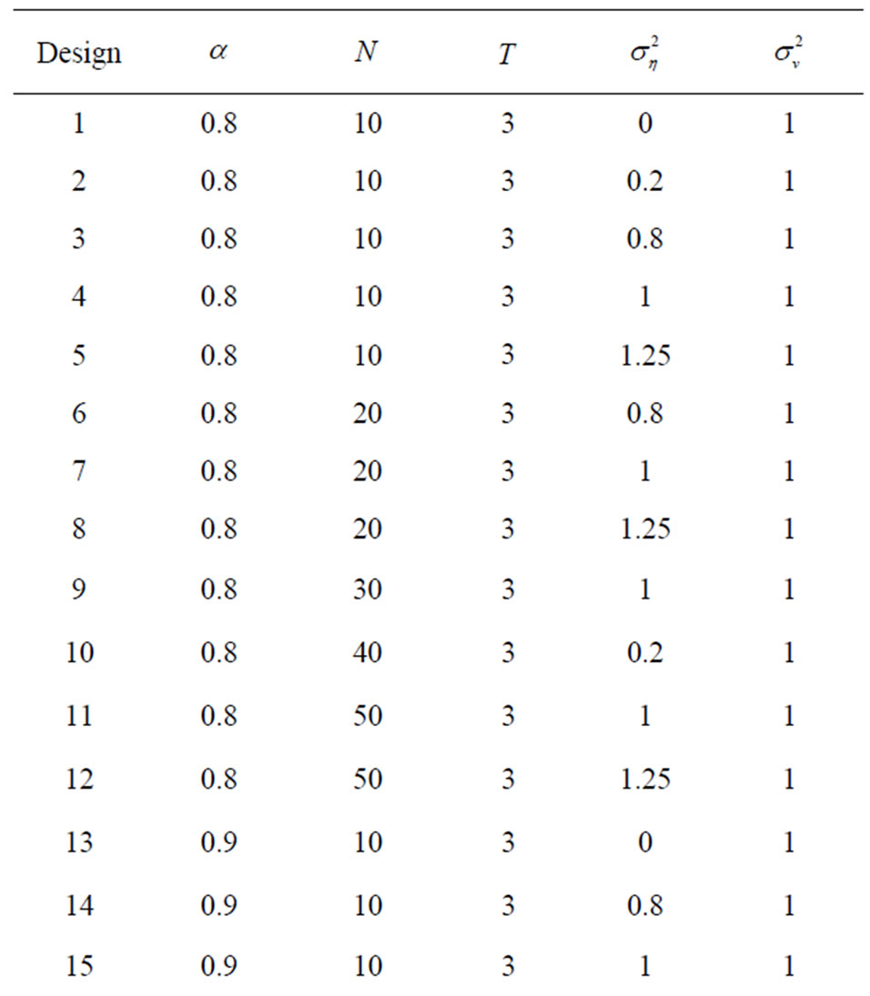
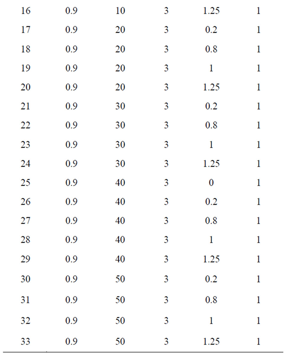
Table 9. Monte carlo designs yielding worst estimates (33 parameter combinations).
The variances of the individual effect for the worst GMM estimates are mostly large, in fact 15 out of the 25 designs considered have  and 21 out of the 25 cases considered have
 . The variances of the individual effects of the 25 worst WG estimates are similar.
When we combine the designs for the 25 largest bias of WG and 25 largest bias of GMM, they have 17 common designs, thus 33 designs in Table 9 represent the worst estimate (largest bias) both from WG and GMM.
The bootstrap methodology is used for these 33 designs. The bias, standard deviation and the root mean square error for the original estimators WG and FDGMM together with the bootstrap estimators WGb and FD-GMM b are presented in Tables 10(a)-(e).
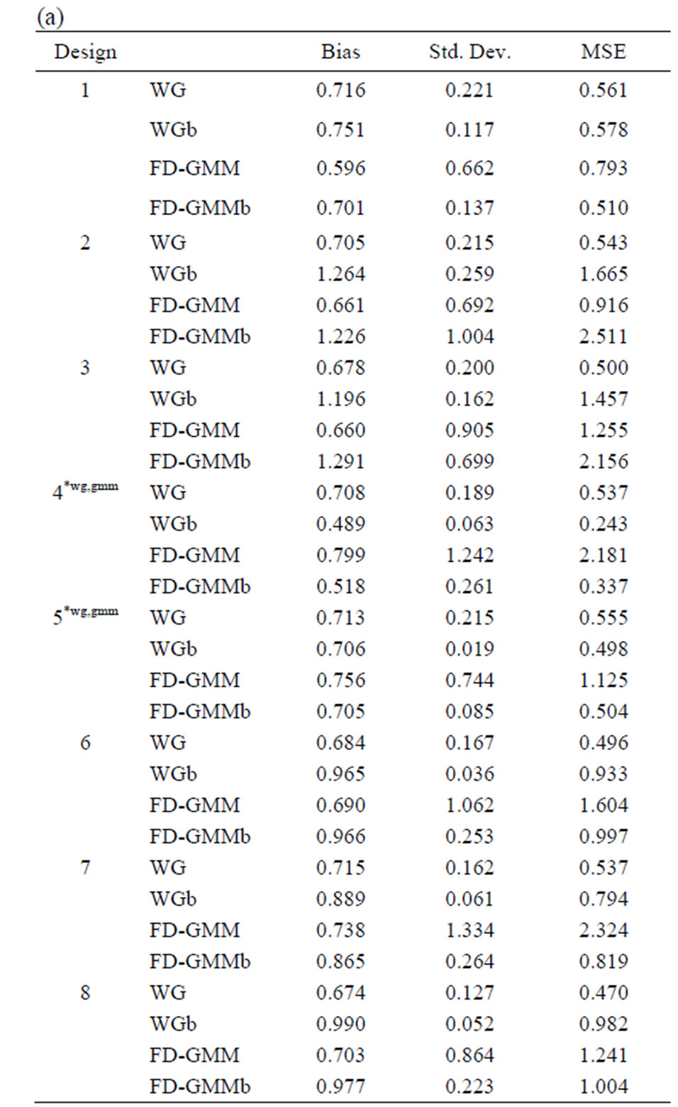
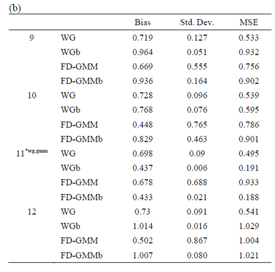
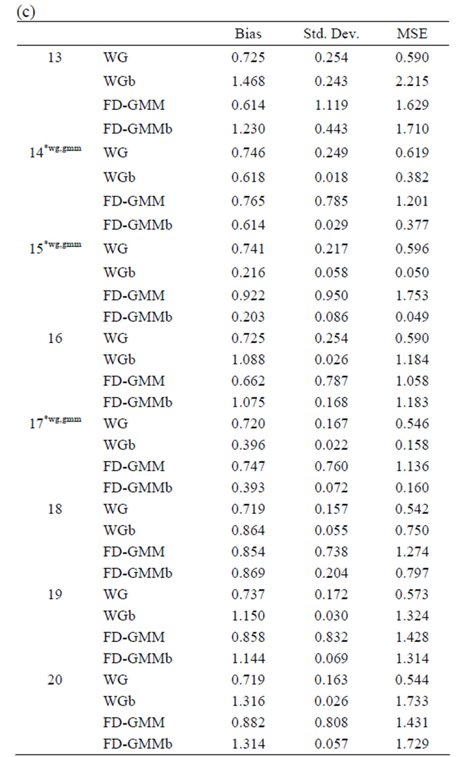
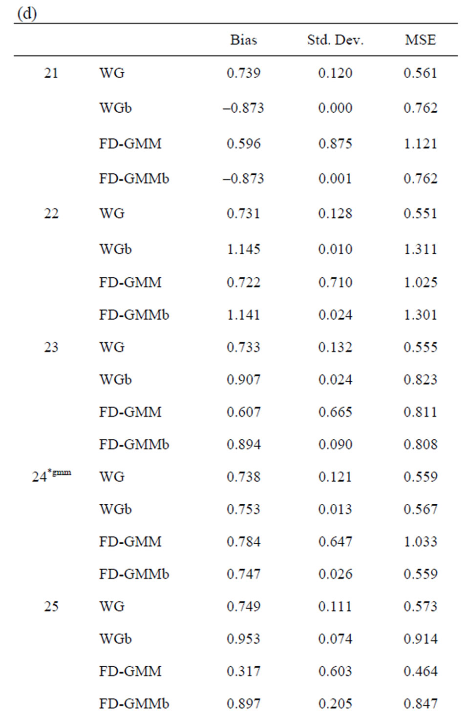
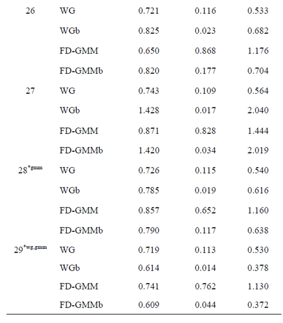
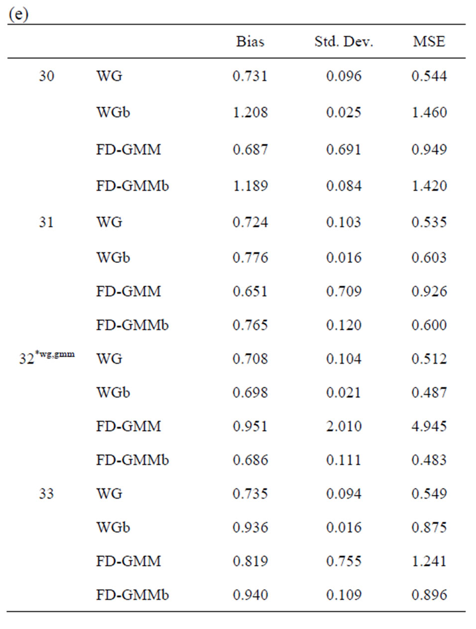
Tables 10. (a) Estimates for  = 0.8, N = 10, 20; (b) Estimates for
  = 0.8, N = 30, 40, 50; (c) Estimates for
  = 0.9, N = 10, 20; (d) Estimates for
  = 0.9, N = 30, 40; (e) Estimates for
  = 0.9, N = 50.
When the true value of the coefficient  is equal to 0.8, the bootstrap estimators WGb and FD-GMMb work well under the smallest sample case scenario, i.e., when
  and
and  where the variance of the individual effect is at least one. Also, for the largest
  and smallest
  combination, i.e., when
  and
and  and the variance of the individual effect is equal to one, both bootstrap estimators perform better than the conventional estimators. The bootstrap estimators for
  are also better than the conventional estimators for the smallest sample case and when the variance of the individual effect is as large as 0.8 and 1.0. However, when
 , the bootstrapped estimators perform as badly as the conventional estimators. Still under small sample case,
  and
and , and time the variance of the individual effect is small but nonzero, i.e.,
  , we obtain the most improved bootstrap estimates for both WG and FD-GMM.
Given moderate size cross-section dimension ( and
and ), the bootstrap FD-GMM is better than the conventional FD-GMM for cases where the variance of the individual effect is as large as 1 or 1.25. Also, the bootstrap WG has smaller bias than the conventional WG when
  and
and .
.
Both the bootstrap WG and bootstrap FD-GMM are better estimators than their conventional counterparts for the largest  and smallest
  case where the variance of the individual effect is equal to one.
7. Conclusions
In estimating a dynamic panel data (DPD) model using WG and FD-GMM estimators, the cross-section dimension  has no effect on the bias of the WG estimator, but the bias of FD-GMM decreases as
  increases in some cases. The bias of WG estimator decreases as
  increases quite consistently in most cases, however, the bias of FD-GMM decreases as
  increases. In square panels such as panels with dimensions, e.g.,
  ,
,  , the WG and FD-GMM estimates are similar. However, when
 , the two estimators are similar only when
 . Also, the WG estimates are similar to FD-GMM estimates for almost square panels such as panels, e.g., (
 ,
, ), (
), ( ,
, ), and (
 ,
, ). When
  regardless of the value of
 , WG and FD-GMM estimates are similar.
WG and FD-GMM estimators are both downward biased, the bias increases with . However, the bias as a percentage of the true value of
  decreases as
  increases. Varying the variance ratio (variance of the individual effect divided by the variance of the random disturbance) does not show sizeable changes on the bias. The bias differs by at most 20% from the approximate bias provided by Alvarez and Arellano (2003) for WG when
  and
and  or when
 . For the FD-GMM, at most 20% bias difference from the approximate large sample bias happen when (
 ,
, and
and ) or (
 ,
, and T = 10, 20).
WG estimates are less variable than FD-GMM estimates based on the interquartile range. The WG estimator is best to use when the time-series dimension is as large as 50 and the cross-section dimension as low as 10 for models where the ratio of the variance of the individual effect to the variance of the random disturbance to be less than one and regardless of the true value of the coefficient parameter. Also, when the ,
,  and
and , the WG estimates are good. These conditions will assure that the percent bias of the WG estimate will not exceed 20%. The FD-GMM estimator has bias not exceeding 20% of the true value of the parameter coefficient for small and moderate samples in terms of
  when: (1)
  and
and , for
, for , (2)
, (2)  and
and , for
, for . The importance of having large
  to reduce the bias and percent bias is evident for designs where the time-series dimension is as large as 25.
The bootstrap estimators for both WG and FD-GMM, labeled as WGb and FD-GMMb respectively, work well for the smallest sample size, i.e.,  and
and  and the extreme sample size set-up where
  and
and , provided that the ratio of the variance of the individual effect to the variance of the random disturbance is equal to one.
8. References
[1] B. Baltagi, “Econometric Analysis of Panel Data,” 3rd Edition, John Wiley and Sons, New York, 2005.
[2] S. Nickell, “Biases in Dynamic Models with Fixed Effects,” Econometrica, Vol. 49, No. 1, 1981, pp. 1417- 1425. doi:10.2307/1911408
[3] T. Anderson and C. Hsiao, “Estimation of Dynamic Models with Error Components,” Journal of American Statistical Association, Vol. 76, No. 375, 1981, pp. 598-606. doi:10.2307/2287517
[4] M. Arellano and S. Bond, “Some Tests of Specification for Panel Data: Monte Carlo Evidence and an Application to Employment Equations,” Review of Economic Studies, Vol. 58, No. 2, 1991, pp. 277-297. doi:10.2307/2297968
[5] M. Arellano and O. Bover, “Another Look at the Instrumental Variable Estimation of Error-Component Models,” Journal of Econometrics, Vol. 68, No. 1, 1995, pp. 29-45. doi:10.1016/0304-4076(94)01642-D
[6] R. Blundell and S. Bond, “Initial Conditions and Moment Restrictions in Dynamic Panel Data Models,” Journal of Econometrics, Vol. 87, No. 1, 1998, pp. 115-143. doi:10.1016/S0304-4076(98)00009-8
[7] J. Kiviet, “On Bias, Inconsistency, and Efficiency of Various Estimators in Dynamic Panel Data Models,” Journal of Econometrics, Vol. 68, No. 1, 1995, pp. 53-78. doi:10.1016/0304-4076(94)01643-E
[8] J. Alvarez and M. Arellano,“The Time Series and Cross-Section Asymptotics of Dynamic Panel Data Estimators,” Econometrica, Vol. 71, 2003, pp. 1121-1159. doi:10.1111/1468-0262.00441
[9] R. Judson and A. Owen, “Estimating Dynamic Panel Data Models: A Practical Guide for Macroeconomist,” Economics Letters, Vol. 65, No. 1, 1999, pp. 9-15. doi:10.1016/S0165-1765(99)00130-5
[10] K. Hayakawa, “Small Sample Bias Properties of the System GMM Estimator in Dynamic Panel Data Models,” Economics Letters, Vol. 95, No. 1, 2007, pp. 32-38. doi:10.1016/j.econlet.2006.09.011
[11] B. Hounkannounon, “Bootstrap for Panel Data,” 2008. http://ssrn.com/abstract=1309902
[12] C. Hsiao, “Analysis of Panel Data,” 2nd Edition, Cambridge University Press, Cambridge, 2003.
[13] C. Hsiao and A. Tahmiscioglu, “Estimation of Dynamic Panel Data Models with Both Individual and Time- Specific Effects,” Journal of Statistical Planning and Inference, Vol. 138, No. 9, 2008, pp. 2698-2721. doi:10.1016/j.jspi.2008.03.009
[14] S. Bond, “Dynamic Panel Data Models: A Guide to Micro Data Methods and Practice,” Portuguese Economic Journal, Vol. 1, No. 2, 2002, pp. 141-162. doi:10.1007/s10258-002-0009-9
[15] J. MacKinnon, “Bootstrap Methods in Econometrics,” The Economic Record, Vol. 82, 2006, pp. S2-18. doi:10.1111/j.1475-4932.2006.00328.x
[16] B. Efron, “Bootstrap Method: Another Look at the Jackknife,” The Annals of Statistics, Vol. 7, No. 1, 1979, pp. 1-26. doi:10.1214/aos/1176344552
[17] P. Buhlman, “Bootstrap for Time Series,” Statistical Science, Vol. 1, No. 1, 2002, pp. 52-72. doi:10.1214/ss/1023798998
[18] G. Everaert, and L. Pozzi, “Bootstrap Based Bias Correction for Dynamic Panels,” Journal of Economic Dynamics and Control, Vol. 31, No. 4, 2007, pp. 1160-1184. doi:10.1016/j.jedc.2006.04.006
[19] H. Chigira and T. Yamamoto, “A Bias-Corrected Estimation for Dynamic Panel Models in Small Samples,” Hi-Stat Discussion Paper Series No. 177, 2006, Institute of Economic Research, Hitotsubashi University. http://hi-stat.ier.hit-u.ac.jp/research/discussion/2006/pdf/D06-177.pdf