Open Journal of Geology
Vol.3 No.6(2013), Article ID:38656,12 pages DOI:10.4236/ojg.2013.36044
Methodology and Equations of Mineral Production Forecast. Part II. The Fundamental Equation. Crude Oil Production in USA
Petro Invest Energy, Houston, USA
Email: sperez@petroinvestenergy.com
Copyright © 2013 Sergio Pérez Rodríguez. This is an open access article distributed under the Creative Commons Attribution License, which permits unrestricted use, distribution, and reproduction in any medium, provided the original work is properly cited.
Received September 19, 2013; revised October 16 2013; accepted October 23, 2013
Keywords: Mineral; Mining; Metal; Oil; Gas; MonteCarlo Simulation; Production Models; Hubbert Curve
ABSTRACT
The fundamental equation of mineral production allows to model and design the dynamics of mineral production, however complex they are or could be. It considers not only the case of a constant production to reserves ratio for given intervals of time, but with a piecewise approach, it is also enabled to account the variation on time of this ratio. With a constant production to reserves ratio, the limit expression of the fundamental equation takes the form of an Erlang distribution with a fixed shape parameter. The rate parameter equals the scale factor. The discrete piecewise version, instead of considering the reserves and the production to reserves ratio being constant through certain intervals of time, updates both variables by units of time. This version, using either lineal or non lineal functions for the variables involved, let to model known production profiles or to forecast them by experimental design. The Hubbert’s linearization updated with recent data and the p-box method applied to determine ultimate recovery of U.S. crude oil reserves indicate official accounts underestimate them. The analysis of the ideal model of production based on Hubbert’s linearization and curve, can be made by decomposing it in the distribution with time of the reserves and of the production to reserves ratio. The distribution of reserves with time is synchronized for both the ideal Hubbert’s curve and real profiles, disregarding whether they match or not. The departure of real profiles from the ideal Hubbert’s curve lies on the differences or correspondences of the distribution with time of the production to reserves ratio. The MonteCarlo simulation applied to forecast US crude oil production for the next five years points to a slow decline, with average annual yields presenting a difference lower than 10% between the start and the end of the simulation.
1. Introduction
In the first part of the present work [1], the equations of mineral production forecast were introduced, showing its capability to model and forecast the production of any mineral, either solid or not, at a widespread range of scales. However, the limitation of a formulation linked to a constant production to reserve ratio through time imposes limits on more general scopes of applications. In the present paper, it will show how such limitations can be overcome, upgrading their field of uses to model and forecast complex patterns of mineral production. In the way, it will show the link between the fundamental equation of the set and Hubbert’s formulas to model mineral production. The classic Hubbert’s method to model or forecast of mineral output presents an ideal trend of rise, maintenance and decline [2,3]. Its difficulties to approach real and complex production profiles led researchers to modify the original concept of the Hubbert model to embrace complicated ranges of production profiles [4]. They tackle the need of both modeling the past and predicting the future of minerals under exploitation. In that sense and scope, during the last decades since the disclose of Hubbert’s proposals [2], the use of its classic methodology for the modeling and prediction of mineral production at large scale has been habitually applied for a diversity of cases. If the ideal and the real profile keep approximately close, as happens with crude oil production in USA [2,3], the Hubbert’s curve fairly succeeds in its task. However, additions and refinements to give it the capability to go beyond archetypal production profiles have also been developed. This situation has led to the development of elaborated methods amplifying the original definition and possibilities of the Hubbert proposal, as the combined generalized Hubbert-Bass model [4] or the probabilistic model of the Hubbert curve [5].
The reason is that outside an initial rough appraisal, ideal models like Hubbert’s are not suitable to be applied directly to replicate or to predict patterns of production where there is a complex profile. These profiles, as we could see in the case of gold mining in Canada (as presented in the webpage 24 h gold), differ from the symmetrical Hubbert’s curve since they display scattered intervals of rises, falls or even average constant values through time.
This raises several questions pending to answers [5], among them, what factors lay deep in the roots of the dynamics of mineral production that makes ideal models to work or not, and how to grasp it?
The methodology and results presented offer answers to such questions. They are based on the link between mineral production and several concomitant variables, provided by the fundamental equation of the set of equations of mineral production forecast [1]. With a novel approach and reformulation, the fundamental equation of the set becomes the fundamental equation of mineral production, able to handle a universal range of production profiles. We shall see evidences of a highly advantageous modeling and predictive tool, whose potential relies, among other aspects, on being capable to lever variation in time of the production to reserve ratio.
We shall see the fundamental equation of mineral production, in its limit expression, offers an (viable) alternative methodology to address this matter, based on the concept of the production to reserve ratio. The EMPF provide the added value of being based on a time related functional relationship between reserves and the rate of production, rather than the classic approach that relies on trend analysis supported by the available data or the more sophisticated and newly arrived methods using elaborated curve fitting by detailed intervals of time. This gives grounds to compare both approaches and to take the best of them to get a more complete picture in order to predict or model mineral production.
The deduction of the EMPF via mathematical induction from the assumptions of a constant PRR, known initial reserves and the law of conservation of matter are departing suppositions. They can be lately treated with flexibility to get insights in cases away from ideal points of departure. In that sense we shall see that a piecewise approach can be set up with the EMPF to model early stages of production, a plateau and even irregular trends, without breaking the core of the postulations behind the EMPF.
The importance of such forecasting techniques is pointed as the wealth of corporations, countries or regions is under scrutiny. Strategic plans rely on production commitments, and among the great urges there is the need of reliable forecasts to be ready to prevent crisis triggered by mineral depletion [6]. As the fundamental equation considers the variations of the PRR with time, addresses the issues of the real dynamics of mineral production. It is capable to yield an exact fitting of production profiles, however complex they could be. This gives a viable alternative to skip the discrepancies between real production profiles and ideal models of production with symmetrical curves. For forecasting purposes, the variables of the fundamental equation can be operated to yield the result on production profiles of different future likely scenarios and conditions.
The modality of research applied to find out the connection between the variables involved in the EMPF is in essence correlational, but once the functional link among the variables is stated, experimental design could take place by inspecting the effects of controlled variables on the output of production or on other variables set up as dependant. Some explanatory research can be ascribed to the elucidation of the meaning of the production as a result of its dependence on the variables included in the EMPF.
General Objectives of the current study are:
To disclose the fundamental equation of mineral production (FEMP); To present evidences of its general character, exposing its universal range of applications to model or predict mineral production; To establish the distribution of PRR with time as a key factor to unravel the dynamics of mineral production; To establish conditions of equivalence between the FEMP and the Hubbert’s curve; To show how the study of the variation of the PRR with time explains whether or not ideal mineral production models match real production profiles; To develop and release a methodology to model or predict complex patterns of production based on the trend analysis of the variables that give shape to the FEMP Specific objectives are:
To analyze the results of decomposing a real production profile in terms of the distribution with time of its reserves and PRR; To apply the link of the FEMP with the PRR to model a selected example of mineral production; To compare a interval of complexity of a classic pattern of production with the models based on the fundamental equation and the one provided by the Hubbert linearization and curve; To provide a comparative example of forecasts based on applying the fundamental equation and the Hubbert’s curve.
And finally:
To provide a full development of the mathematical background behind the fundamental equation of the set of EMPF via mathematical induction (in Annex 1), The procedure followed in the development of the current project first consist on the set up of the theoretical basis and then on the unraveling and application to the case under study of a practical methodology based on these results.
2. Set up of Theoretical Basis
This section embraces:
1) Derivation of the fundamental equation of mineral production (from the fundamental equation of the set of EMPF);
2) Set up of the discrete piecewise version of the FEMP;
3) Comparative study between the FEMP and the Hubbert’s curve.
2.1. Derivation of the Fundamental Equation of Mineral Production
Lets first recall the starting set of the Equations of Mineral Production Forecast (EMPF):
The fundamental equation of the set of EMPF, as introduced in [1], is the first one of a set comprising the following:
 (1)
(1)
 (2)
(2)
 (3)
(3)
where:
n: years of production;
R0: volume of original reserves;
 : production at the nth year;
 : volume of remaining reserves at the nth year;
C: average production to reserves ratio;
 : Cumulative production at nth year.
For the purposes of the present study, the productionreserves ratio (PRR) for every year is defined as the respective production of that year divided by the reserves available at the beginning of the year. In the equations, it will be designated with a capital C.
The Fundamental Equation of Mineral Production
“Eternity lasts no time” [7].
Let’s consider an examination of Equation (1) applied in a piecewise fashion. This can be done by using it at intervals of time where the data of remaining reserves is updated at the start of each interval and time is reset to one at the beginning of the interval:
Be Ri−1 the value of the estimated reserves at the beginning of a period (i) covered by the piecewise function. Notice it is used the sub index i − 1 to follow the fact the reserves precede the beginning of production at every interval.
If  means the production at the first year of the period, we then have a consequent PRR as:
 (4)
(4)
As reserves varies from year to year due to revisions, discoveries or other reasons, at year n it is proposed the use of a factor  that will adjust the reserves
  at the beginning of the period:
 (5)
(5)
But at year n, by applying the factor  to adjust the reserves, we will also have a modified PRR:
 (6)
(6)
So, as stated by Equation (1), by year n the production  corresponding to the reserves adjusted by the factor
  will be:
 (7)
(7)
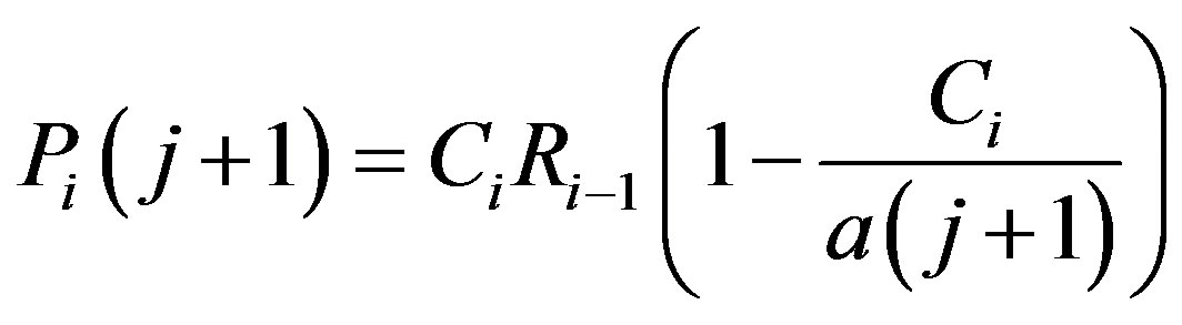
To simplify the results of the following deductions, a change of variable, n = j + 1, allows to conveniently get n − 1 = j, so Equation (7) becomes
 (8)
(8)
Further examination of Equation (8) lead to consider what would happen after n years of production. Most likely, with enough time running, the update of the depleted reserves would involve a decrease from the initial amount Ri−1. In this case  handles the proportion of the decrease.
Become aware, for the sake of the following deduction, that there are conditions where if the reserves are developed beyond certain degree, as n increases, then  most likely should decrease.
It is found [8] the following limit of Equation (8) when time goes to infinity  and
and  goes to zero
 :
:
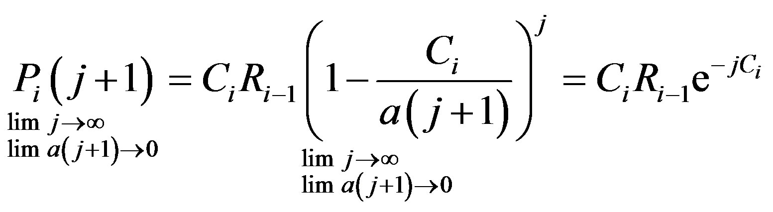 (9)
(9)
For each interval of time considered, Equation (9) can be seen as an Erlang distribution with a fixed shape parameter. The rate parameter equals the scale factor [9].
Equation (9) gives a general law linking mineral production of an interval of time with time itself, the reserves at the beginning of the interval and a constant production to reserves ratio over the interval. It can be quoted as:
The profile of the production with time equals the multiplication of a scale factor  by the natural exponential number (e) raised to the multiplication of the negative value of time by a ratio of the scale factor. The ratio is the scale factor divided by the reserves available at the start of the interval of time
 .
.
Notice when j = 0 then n = 1, and at the very first interval (i = 1), the production at year one equals the multiplication of the PRR by the initial reserves R0, as stated in Equation (1), since e0 = 1.
Notice also that for every new interval after the very first, the first production of the interval can be obtained setting up j to zero.
Equation (9) can be viewed as a platform to introduce the notion of reserves and of PRR as time dependent functions. To that end it is enough to account with a dynamics of production comprising several consecutive intervals of time of arbitrary lengths with the reserves and the PRR following a functional law over the intervals. Going further, even if each interval of time is reduced to be of unit length, there are several ways to set up functional connections between time and the distributions of reserves and of production to reserves ratios. Polynomial fitting, to quote one example, is one of these ways.
Lets design them as  and
and , respectively.
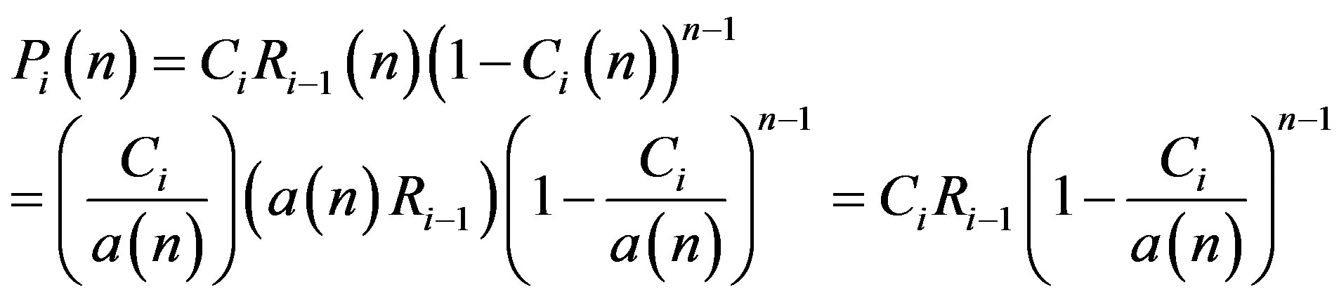
So, for a piecewise discrete approach (with unity as time interval), Equation (8) can be reformulated as Equation (10) and quoted as:
The profile of the production with time equals the multiplication of a time dependent scale factor  by the natural exponential number (e) raised to the negative value of a ratio of the scale factor
 . The ratio is the scale factor divided by the reserves
  available at every
  -th discrete point of time
  .
.
The scale factor is directly proportional to the (linear or non linear) time dependent function of the PRR. The constant of proportion is the reserves available at every discrete point of time.
2.2. Set up of the Discrete Piecewise Version of the FEMP
The use of Equation (9) in a piecewise manner can be thought in two ways. In one it is applied in discrete intervals of time. In another, each discrete interval of time are reduced to length one, and then Equation (9) becomes:
 (10)
(10)
As with this particular approach the Reserves and the PRR are updated every time, we have found an alternative way to get a time dependent expression of the Fundamental Equation without breaking the core of the postulations behind the EMPF.
The simplicity of Equation (10) could mislead and conceal its extraordinary capabilities to model historic distributions of production data or to forecast future trends. We shall see how it is suitable to be applied to accomplish both goals. But first, the reader is invited to explore in the next section the connection between Equation (10) and the formulas of the Hubbert’s curve and linearization.
2.3. Comparative Study between the FEMP and the Hubbert’s Curve
For the use of this article, is understood that initial reserves R0 is equivalent to the expression of ultimate recovery Qt, and PA equivalent to the cumulative production Q as meant in the formulas of the Hubbert’s curve and linearization model [3].
Lets establish what is the nature of the PRR as implied by the Hubbert’s model. The linear expression of the PRR through time, as offered by the logistic curve for the case under study, is a reflection of a more general feature of this model:
Since:
 (11)
(11)
Then, to obtain the PRR from the expression of the Hubbert’s linearization [3] it can be done in two steps as follows:
First, a rewriting and rearrangement of the variables of the expression for the Hubbert’s linearization of production lead to:
 (12)
(12)
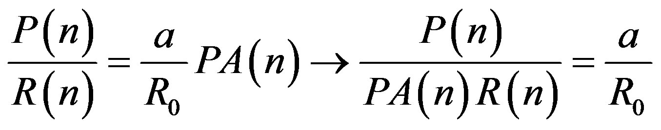
Second, we come out with the construction of an expression for the PRR based on the division of Equation (12) by Equation (11)
 (13)
(13)
So, the Hubbert’s curve, as stated by Equation (12), result is a PRR with a constant linear rate of growth given by multiples of the ratio .
.
Notice in Equation (13), although equivalent to Equation (10), there is synchronization of the time index for all the variables. In effect, the definition of Equation (11) allocates  and Equation (12) assigns P(0) = 0. From Equation (13), it is seen that the PRR as implied by the Hubbert’s curve is a linear function of the cumulative production. The slope of the line is the ratio of the “a” intercept [1] to the initial reserves R0. Equations (10) suggest to rethink the Hubberts curve as one composed by the multiplication of two intervening factors, the PRR and the reserves.
Equations (10) and (12) allows to rewrite the Hubbert’s curve with the piecewise discrete version of the fundamental equation (Equation (10)) in terms of the ratio , and the distribution with time of the reserves and the cumulative production:
 (14)
(14)
So, the Hubberts curve, with the parameters of the ideal profile of production, is implicitly formulated in the expression of Equation (10) and vice versa. By splitting the formula of the Hubbert’s curve in the contribution of the two factors found, we can address the question of the departure of ideal from real profiles. We shall see that at time n, the difference between the ideal and the real profile comes by the difference between the real and the ideal production to reserves ratio.
3. Methodology and Results
Once the theoretical basis is determined, it is convenient to proceed with the application of the abstract results to the cases to be studied following the next general procedure:
1) Estimation of R0. The working scale is a fundamental factor to decide a methodology to follow to determine R0. If the case of study consists of individual reservoirs, R0 can be estimated by several techniques supported by a geologically driven appraisal [10-13]. If the working scale includes several reservoirs, and their combined picture present an early development of mineral resources, where the Hubbert’s linearization is not the best choice to apply, probabilistic approaches are of common usage [5,14]. The Hubbert’s linearization [2,3] can be applied if the degree of development of resources is advanced enough and the working scale is greater than individual reservoirs (fields, basins, corporative assets, countries, regions, etc.). In this latter case, in the plot  versus P, use peak points of the dataset to define an envelope or range of values. This will help to identify a lower, an average and a upper estimate of R0.
2) Having R0, the historical distribution of the reserves and the PRR with time are determined. Equations (9) and (10) are applied if there is requested to model the historic distribution of production. Equation (9) works for intervals where the PRR keeps a constant profile, otherwise Equation (10) comes into use.
4. To Forecast Future Outputs of Production the Procedure Is as Follows
1) From a suitable starting point, count the points above, on and below an average line inside the envelope of the dataset. They provide the statistical input for the assignment of probabilities of occurrence of the upper, middle and lower estimates of initial reserves. References of this way to assign probabilities according to the distribution of points inside the extrapolation of an envelope of data could be found in [15-17]. In the current study, it will be of ample use for the analysis of correlation between variables with dispersion of data not easily modeled by conventional means.
2) With the real data of production, and using the official, the upper and the lower estimates of initial reserves, build up two sets of distribution with time, one of reserves and another of the PRR.
a) Modeling of the distribution of reserves. Using the dataset obtained in (2), and the method explained in [1], the statistical parameters (average, standard deviation, coefficient of variation) of the distribution of reserves are found. For the years to simulate they are useful to set up a normal distribution. The definition of proven reserves also lead to restrict the distribution to a range of values from 90% to 110% around the average.
b) Review and modeling of the distributions of PRR. The last trend the data outline can be used to get a window of future values inside an envelope or P-Box [17]. As described in the first step of the methodology, the envelope could be also based on the peak points encompassed by the set. Again, the distribution of points inside the envelope of the dataset provides the statistics for the assignment of probabilities of occurrence of the upper, middle and lower estimates of the PRR 3) If from the previous analysis the future tendency of the PRR is to be kept as a constant value, use Equation (9) and the method presented in [1] to calculate the output of production. If the analysis indicates the PRR is not constant, use Equation (10) and a probabilistic range of PRR inside the envelope devised to forecast the production. Discrete probabilities of occurrence, based on the counts made from the average line inside the envelopes are assigned to the factors in Equation (10) to give its imprint to the simulation runs. The MonteCarlo simulation provides probabilistic forecasts, as illustrated in [1], giving a bidimensional picture of the likely outputs of production.
Case Study: Crude Oil Production in USA
With the purpose of introducing the analysis of production oriented to the value of understanding their dynamics lets take Oil production in USA as our case under study. USA’s crude oil production is considered not only as an example of a fair match with the Hubbert’s curve model [3], but also an interesting arena to apply models to match disruptions or differences with ideal profiles [18]. So, this versatility makes it an appropriate case to display the connection of the Hubbert’s curve with the FEMP. The input data for the following results comes from an official source [19]. The first step is the diagnosis of a range of the initial reserves, or ultimate recovery, using an approach based on the Hubbert’s linearization. To that end will suffice the extrapolation of an envelope of the distribution of points of the plot of cumulative production versus the ratio of production to cumulative production. In Figure 1, the points from 1958 to 2012 are used to make this task.
The upper boundary (black segmented line) rest on the peak points of 1970 and 2012. The lower boundary (green segmented line) is aligned with the peak points of 1976 and 1999. They point to 235.8 and 256.3 billion barrels of ultimate recovery (initial reserves), respectively. The line of bet fit of the whole distribution (brown segments, Figure 1), keeps inside the envelope for most of its length but intersects the lower boundary by its indicated value of ultimate recovery.
Our next task is to show how to use Equation (10) to model the historic distribution of production outputs, especially in those intervals of time where the real profile departs from ideal models. To illustrate the case, lets examine the distribution of reserves and of the PRR of the last ten years, based on the upper value of R0 (256.3 BB) according to the results of the envelope of the Hubbert’s plot. During that interval of time there is a clear break that complicates the classic production profile of crude oil in the US. The figure next to the last of the present work includes the complete profile and this example.
First, notice how the two independent variables considered in Equation (10) are fully featured with the known data of production and the estimate of R0.
Once a figure of initial reserves R0 is determined, the remaining reserves at every year are given by subtracting the cumulative production from R0. The chosen R0 could be given by the envelope on the Hubbert’s linearization plot as indicated in Figure 1.
The first aspect to consider is the match between the ideal a real distribution of reserves with time (Figure 2). But the same does not happens with the historical and the
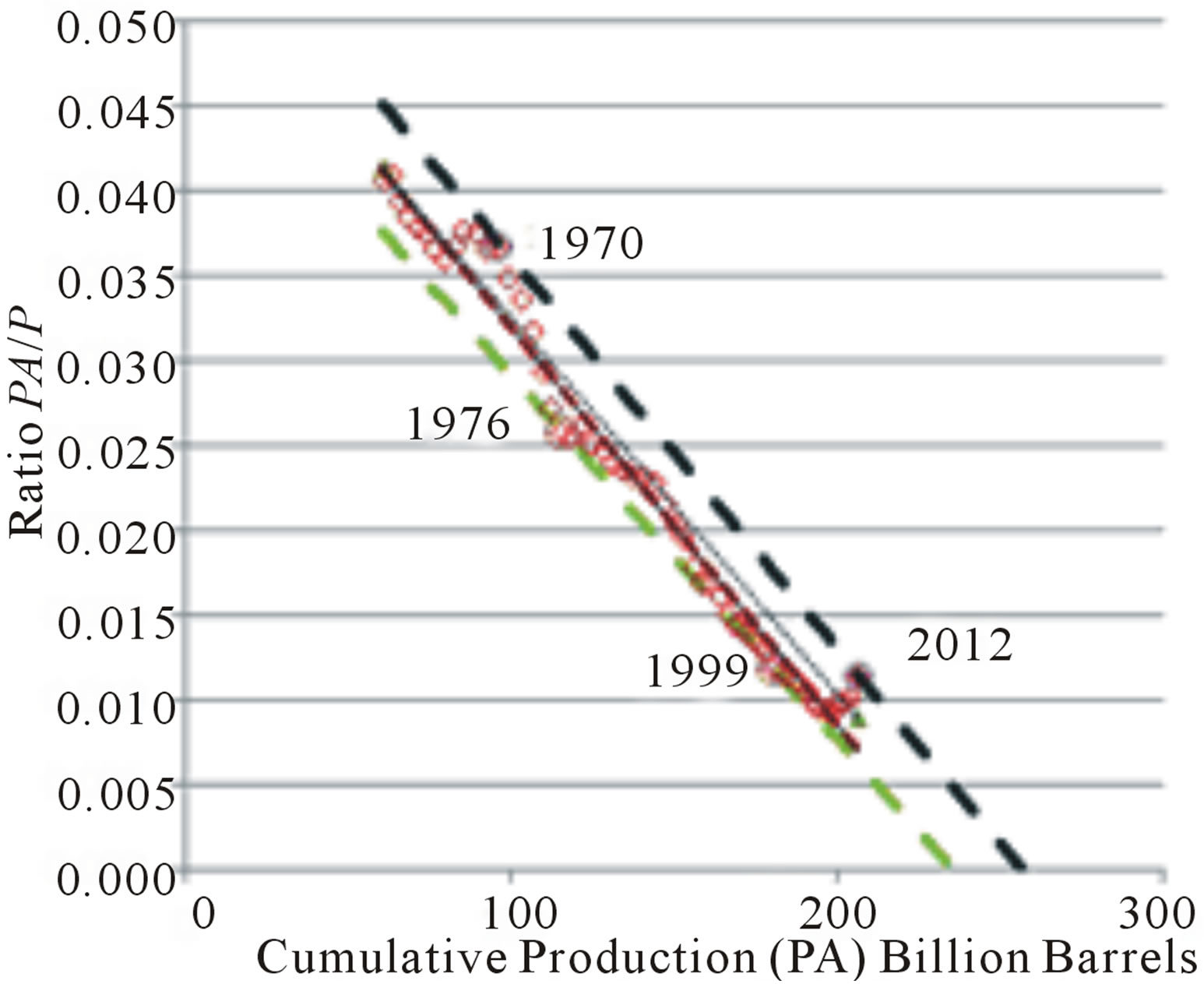
Figure 1. Hubbert’s linearization plot with an envelope to determine a range of the initial reserves R0.
ideal distribution of PRR (Figure 3), derived from the historical and ideal ratios of production over corresponding remaining reserves.
A third degree polynomial fit of the real PRR (brown segments) could provide the input in Equation (10) to model the real ratio. In other circumstances of departure of the ideal and real profiles, the model of the real PRR could even be linear. The case observed is non linear, but readily to be divided in two near linear segments with a pivot point in 2008.
The exact match between the historic data of U.S. crude oil production and the concomitant distribution of points is given by applying Equation (10) considering the models of the distribution with time of the reserves and of the PRR. In the latter case, as indicated previously, a low degree polynomial fit will suffice.
Let’s proceed with the simulation to forecast the future trend of production. The assignment of probabilities of occurrence of determined values of reserves during the simulation of production could be based on the count of points above and below a split line inside the envelope. One option for the split line could be the average or mid-
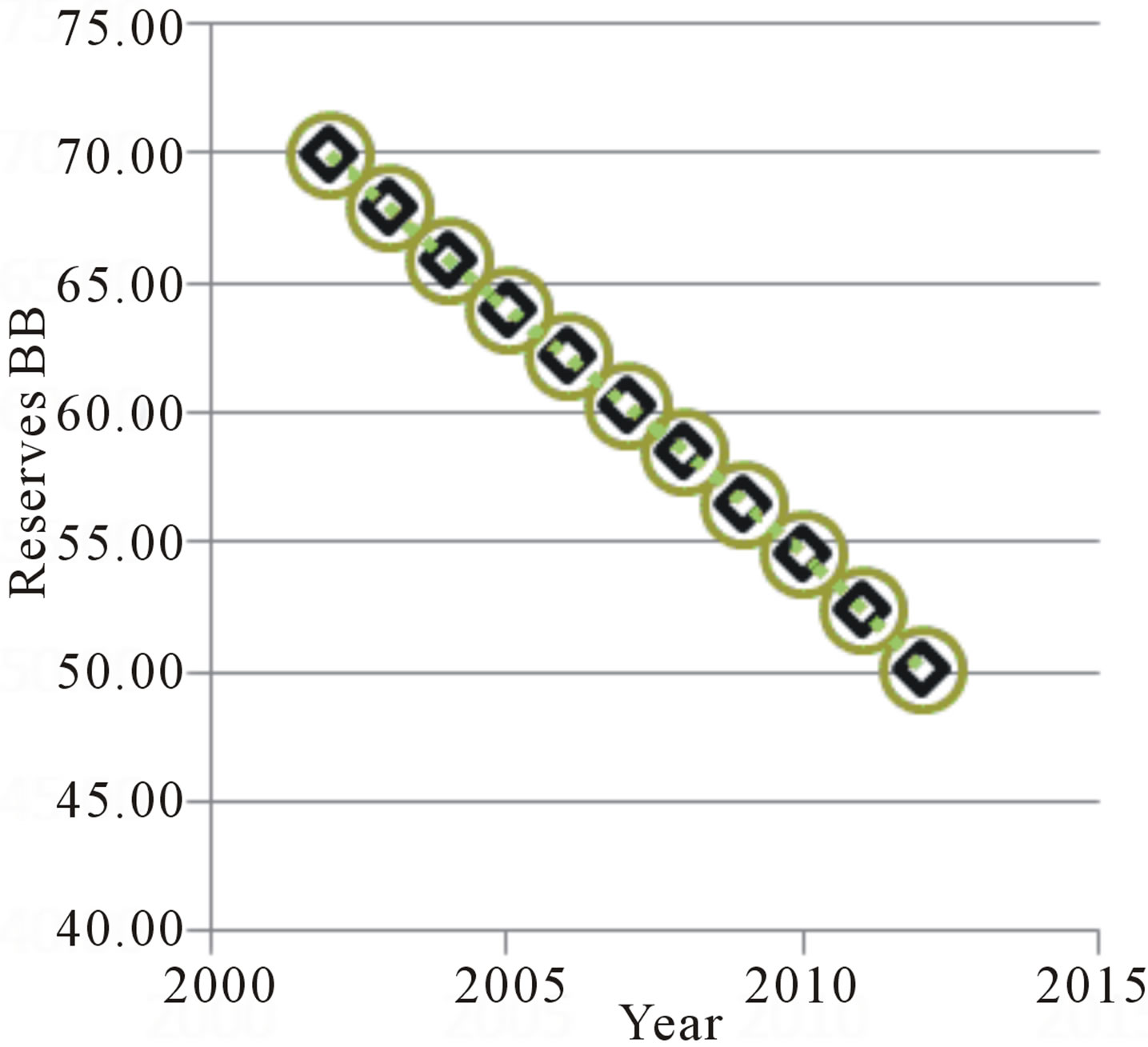
Figure 2. 2002-2012 crude oil reserves in USA. Ideal (black squares) and real (green circles) distribution with time.
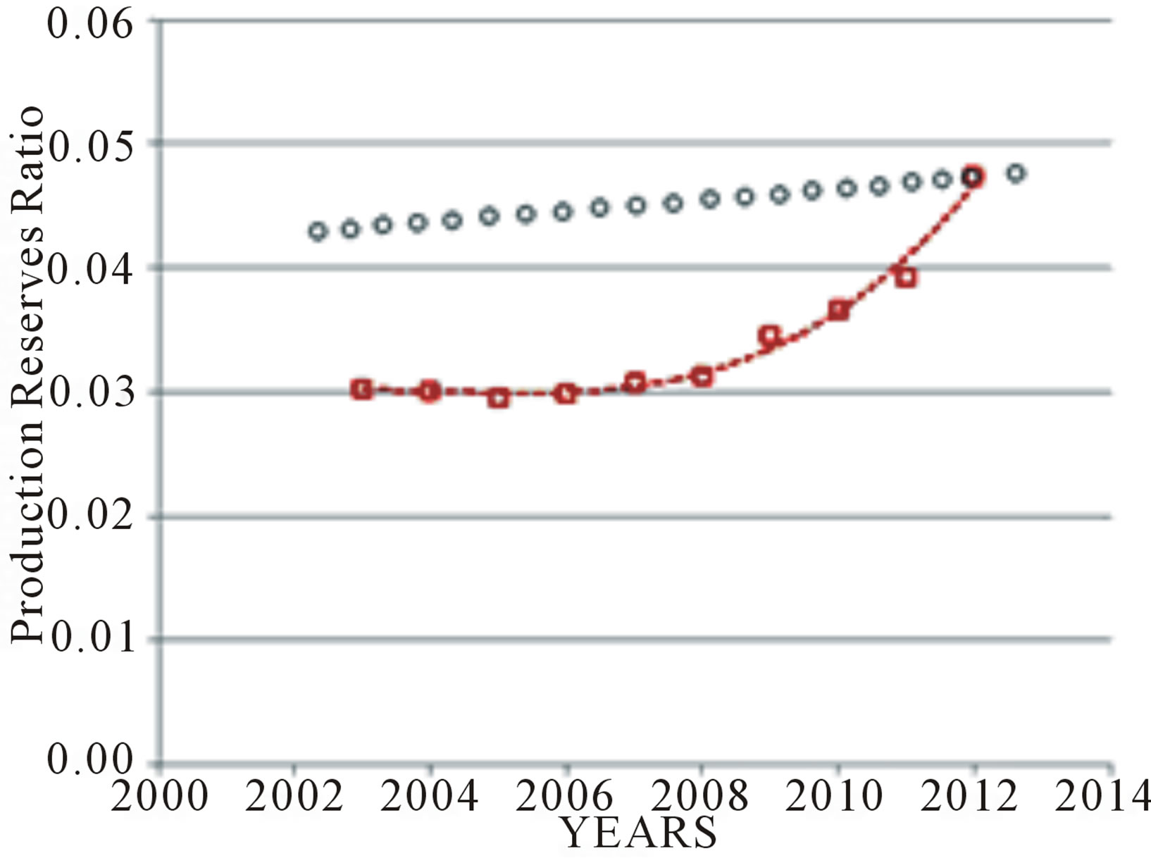
Figure 3. 2002-2012 PRR of crude oil production in USA. Ideal (black circles) and real (brown squares) distributions with time.
dle line inside the envelope, another line of best fit.
Under this viewpoint, in the first case the probability of occurrence of reserves is 78% biased to the lower end, while is around 22% inclined to the upper end. In the second case the bias is 66% and 34% to the upper and lower ends, respectively. So, the first result, with a bias higher to the lower end of values than the second gives an optimistic, and the second a conservative, estimate of reserves. Let lwb and upb designate the fractions corresponding to the percentages of the aforementioned lower and upper bias. Let  and
and  be the remaining upper and lower ends of the reserves at year n, for either the conservative or the optimistic estimates. Then, the probabilistic average of reserves for every year
  for either the conservative or the optimistic alternatives is calculated by
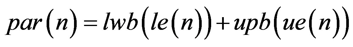 (15)
(15)
The results provided in the following paragraphs are based on the average of the optimistic and conservative values of reserves, what means
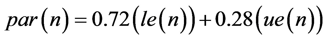 (16)
(16)
In Table 1 are summarized the results of the study of likely value of U.S. reserves by the year 2012 according to the previous statements.
The method will focus on the analysis of the Hubert’s curve under the viewpoint of Equation (10), the discrete piecewise version of the FEMP. As we recall from Equation (14), the Hubbert’s curve can be decomposed in the product of the ideal distribution with time of the reserves and of the production to reserves ratio.
By examining in Figure 4 it is seen that disregarding the upper or lower end, the ideal and real distributions of the reserves with time have a perfect coincidence between them.
The almost linear, high slope trend of reserves depletion observed since the second half of the last century was preceded by a slower pace of depletion that changed in the neighborhood of WWII.
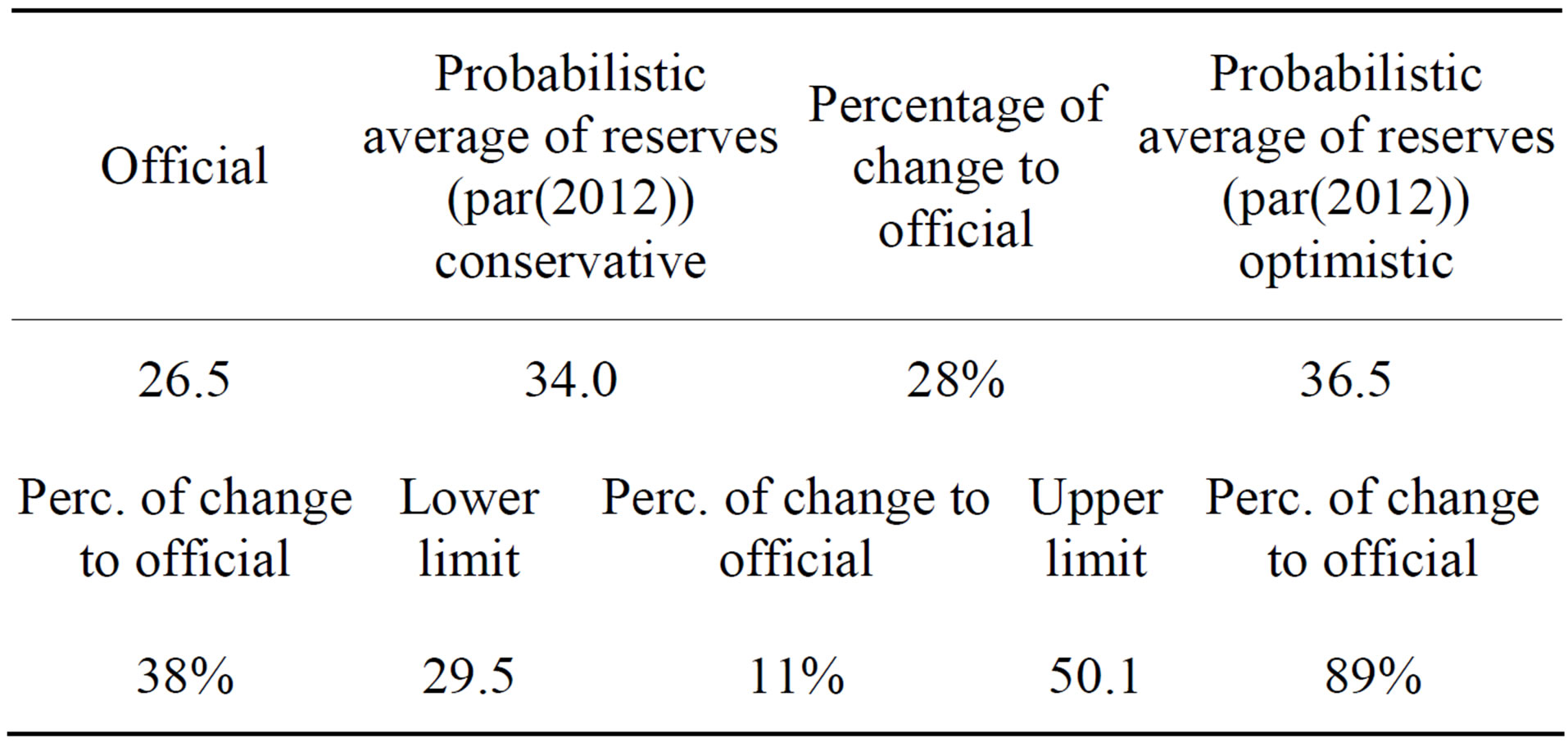
Table 1. Year 2012. Figures in billion barrels. Comparison between reserves according to official sources and as indicated by the upper and lower limits of the envelope of the Hubbert’s linearization plot.
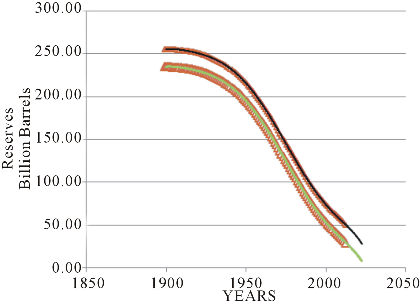
Figure 4. Distribution of reserves with time. Comparative plot of the real (brown dots) and the upper and lower Hubbert’s ideal distributions (black and green traces inside brown dots, respectively).
For the simulation of production according to the method presented in [1], the official data of reserves will be used to raise concomitant statistical parameters. A Weibull distribution was selected from the set of best fitted distributions to the historical data of reserves (2002-2012), following the criteria offered in [1] and also considering the highest minimum value supported by the ideal fit (around 18 billion barrels). In Figure 5 is seen the histogram and best curve fit of the historical data of reserves for the decade 2002-2012. The mean value has 90% chance of being between 19.12 and 26.54 Billion Barrels The coefficient of variation indicates one standard deviation of the data oscillates 9% from the mean.
But when the real and the Hubbert’s ideal distributions of PRR with time are compared some issues are raised.
First, notice the onset of changes in the trends of both variables is not coincidental. For instance, there is no a remarkably change in the slope of the PRR with time in coincidence with the sharp increase in the depletion of reserves with time appreciated by the middle of the last century Second, the ideal and real trend of the PRR is not fully concurrent as in the case of the reserves. Both trends follow a rather close pattern up to the early seventies of the last century. Since then, the real distribution presents intervals where the PRR either:
Steps away from the ideal Hubbert’s profile, following a near constant value with time (1971-1976 and 1985- 2005);
Keeps a tendency to follow Hubbert’s ideal profile (1976-1985);
Or to reach again (2007-2012) the ideal Hubbert’s profile.
So, as far as concerns the comparative analysis of the two factors that characterizes the real and the ideal production profiles of the USA crude oil production, differences, if any, are seen only reflected in the distribution with time of the PRR (Figure 6).
The two end limits for ultimate recovery (or R0) as given by the Hubbert’s linearization analysis can be used to model likely ideal patterns of production.
The distribution of real data is then confined inside the envelope provided by the ideal curve boundaries (Figure 7).
In the case of crude oil production in USA, both ideal curves fairly match the real distribution up to the 50’s of the last century. Since then, the lower boundary catches up the low end outputs of production of the real distribution, while the upper boundary confines below those points above the lower boundary.
The 2013-2018 forecast of averaged outputs (brown circles) and estimated from official reserves (blues crosses) are displayed with the years in labels. They were obtained by applying Equation (10) and the methodology for stochastic forecast outlined previously.
A bidimensional forecast, or summary graph, can be produce with the aid of the software @Risk, after running the MonteCarlo simulation in microsoft Excel.
The yellow line in Figure 8 indicates the most likely
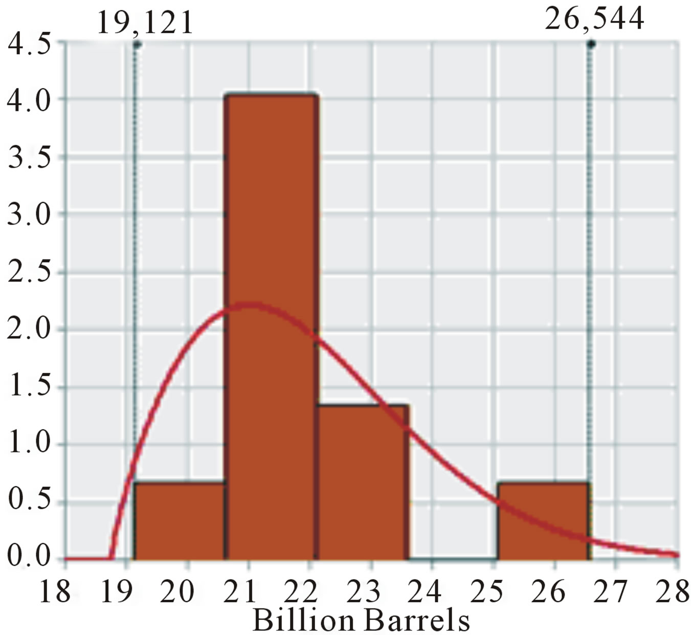
Figure 5. Historical data of crude oil reserves 2002-2012. Histogram and best curve fit.
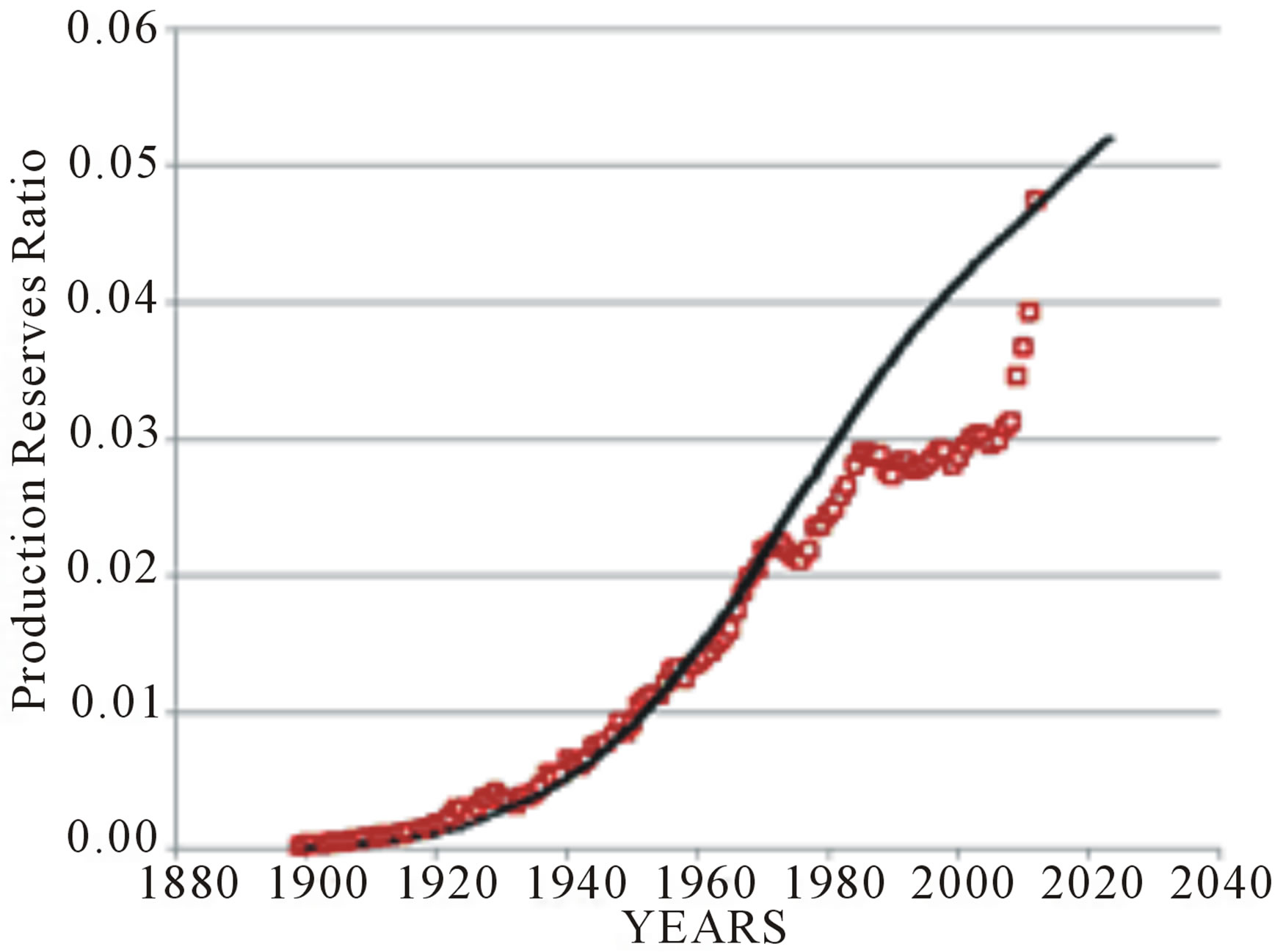
Figure 6. Upper end of R0. Distribution of PRR with time. Comparative plot of the real (brown circles) and the Hubbert’s ideal (black points) data.
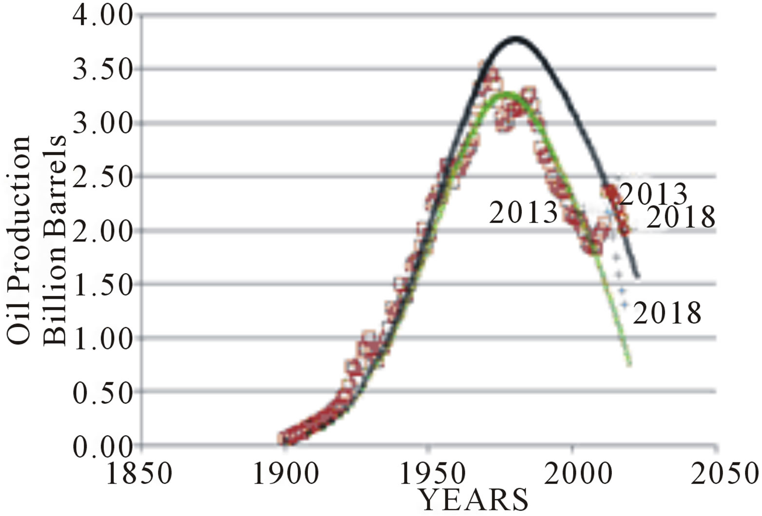
Figure 7. The upper and lower ideal Hubbert’s curves of production (black and green intertwines, respectively) as they side with the real historic distribution of US production data (brown squares).
or average outcome of oil production after running the MonteCarlo simulation according to the settings provided to the variables of the EMPF.
The statistical record of outputs of the simulation allows to make probabilistic intervals of confidence for the mean value of the production for every year. The inner interval provides a interval of confidence one standard deviation above and below the average value where the simulation converged. So there is around 66% of probability the size of the output of production inside this inner band. The outermost band provides 90% of probability for the interval of confidence.
For the purpose of the simulation of production, the reserves as stochastic variables are modeled with two main controls. One is the coefficient of variation determined from the statistical analysis of the data. The first the limit imposed by the definition of proven reserves. In this latter case the stochastical distribution is set to be confined between a fraction between 0.9 to 1.1 times the average value.
So, taking advantage of working with two dimensional forecasts as in Figure 8, lets appreciate the range of values the production could end up under a probabilistic window. First, the probabilistic forecast based on the method explained is featured by the yellow line inside the grey bands.
It is also seen an upper and a lower ideal Hubbert’s curves of production (black and green segments, respectively) confining the production estimated from official reserves (blue line).
For instance, for 2013 there is 90% probability the production of oil between 1.28 and 3.52 Billion Barrels, with an average value of 2.40 BB given by the yellow line. By 2018, although the average value drops to 2.25 BB, the 90% probability window is wider than in 2013. As a result, there is 90% probability the production in 2018 be between 0.65 and 3.75 BB. The difference between the average values between 2013 and 2018 is less than 10%, an indication of a slow decline for the interval
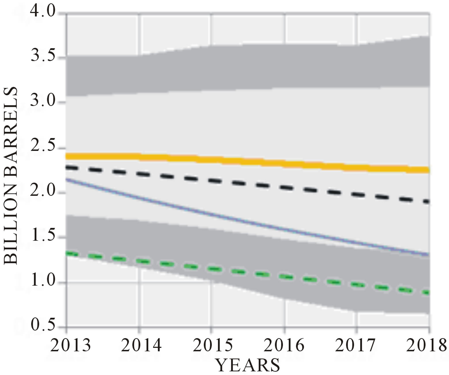
Figure 8. Probabilistic forecast of US crude oil production (yellow line inside grey bands).
under study.
Both the Hubbert’s curve for a total recovery of 256 BB (HCTRU, black segments) ,and the estimated production based on the official recovery of reserves (HCTRD, blue points), keep inside the lower side of the 66% probability window from 2013 until 2018. The Hubbert’s curve for a total recovery of 235 BB (green segments) stays inside the lower side of the interval between the 66% to 90% probability window. The estimated production based on the official recovery of reserves departs from the HCTRU to approach the HCTRD from 2013 to 2018.
5. Discussion
The dissection of the formula of the Hubbert’s curve in the variables that define Equation (10) paves the way to understand the difference between the real and the ideal dynamic of mineral production.
The readers are invited to compare models based on the FEMP with other proposals achieving the same goal. The use of the FEMP relies on the real distribution of the PRR with time as a single time dependent variable to correct departures of ideal from real profiles. In other valid proposals [4,18], there are at least two variables to input the control on how far the production decreases (or increases) below (above) the ideal, and how quickly the production recovers (declines) toward the real. Time is an additional explicit variable. The distribution of the PRR with time collapses in one single set of variables such corrections.
Regarding the use of Equation (10) to model the historic distribution of production, it can be argued that in shape of the variable PRR there is a circular reference to the object of the model, the production itself.
This can be sustained if Equation (10) were applied year by year, without formulating any mathematical conjecture of its behavior with time. But this is not the case, since it is considered the piecewise modeling of the distribution of production working by intervals using as a reference a functional fit of the distribution with time of the PRR. A polynomial or other suitable approach for the fit will model the distribution of the PRR with time, as shown in the example of Figure 3. The intervals of the piecewise model could account with linear or non linear fits of the change of the PRR with time. For intervals where the PRR is constant, the direct use of Equation (9) is viable. As to calculate the component of distribution of reserves with time is synchronized for both the ideal Hubbert’s curve and real profiles, disregarding whether they match or not. This is a consequence of how is built the interpolation in time of the cumulative production for the Hubbert’s curve. In Equation (10), the input for the Hubbert’s curve of the distribution in time of the reserves is given as in the real profile. It consists of the straightforward difference between the initial reserves and the cumulative production with time. But the input of the PRR to the Hubbert’s curve, as indicated by Equation (12), takes a direct proportion of the distribution of the cumulative production with time for this factor. The constant of proportion being the ratio . The ideal and real PRR will coincide as far as the ideal PRR coincides with the corresponding real ratio of production to reserves, but as the latter obeys the control on the dynamics of production of issues. In a formula, for both PRR to coincide must occur that at every simultaneous point of time the ratio of the production to the multiplication of the cumulative production by the reserves be constant. The constant equals the ratio of the “a” intersection of the Hubbert’s linearization model to the initial reserves:
 (17)
(17)
The departure or coincidence of real profiles from the ideal Hubbert’s curve lies on the differences or correspondences of the distribution with time of the production to reserves ratio.
From Equation (10) it is inferred the production can be envision as a composite function of the distribution with time of the reserves and the PRR.
The envelope used to extrapolate the PRR of crude oil in USA widens with time. This enlarges the size of the probability window for oil production in the country from 2013 to 2018.
The focus on the analysis and projection of the trend of the PRR component of the fundamental equation to forecast future outputs of mineral production has caveats. First, the dependence of the production output to the variables involved in the fundamental equation changes according whether Equation (9) or Equation (10) are considered. In the first case, although for every interval the PRR and the initial reserves are constants and the only variable that changes is time, it is also true that for the whole picture of a simulation it will be noticed the variation of the aforesaid constants from one interval to the next. In the second case time is always constant and is set up to zero. The variables that change are the PRR and the reserves. In both cases a sensitivity analysis of the response of the production output to the independent variables is recommended as a way to ponder they relative weight on the dependent variable. Further studies will provide insights on the connection of the variables of the FEMP and aspects as cycles and sub-cycles presented in the yield profiles of minerals [20,21].
6. Conclusions
The FEMP, in its expression as an Erlang distribution, offers an instrument to model mineral production when there is a constant PRR over the interval of time considered. The piecewise discrete version, presents the complementary resource to model mineral production when the PRR is not constant with time.
The formula of the Hubbert’s curve of production can effectively be divided in the contribution of the distribution with time of the two variables considered in the FEMP. They configure ideal distributions of reserves and PRR, leading to a symmetrical curve of mineral production.
If a profile of mineral production is analyzed looking at the variables of the FEMP, the difference between the real and ideal profile is only reflected in the PRR. The ideal and real distributions of reserves with time always match.
The general capability of the FEMP to model historic profiles of production, however complex they could be, relies on fitting the distribution with time of the PRR, as independent variable, to an adequate linear or non linear trend. This gives a viable alternative to skip the discrepancies between real production profiles and ideal models of production with symmetrical curves.
The coincidence of ideal and real distributions of reserves with time leaves to the other variable of the FEMP the role as the key variable to ensure the match (or discrepancy) between the ideal and the real production profiles. As the fundamental equation considers the variations of the PRR with time, addresses the issues of the real dynamics of mineral production, the factors affecting the dynamics, disregarding what they could be, are truly reflected in the PRR.
For forecasting purposes the variables of the fundamental equation can be probabilistically operated to yield the result on production profiles of different future likely scenarios. An adequate connection between the behavior of the PRR and the diversity of factors that decide the dynamics of production (political, economical, others) is central to ensure the proper prediction of this variable and of the forecast of mineral outputs.
7. Acknowledgements
To my patroness and patrons for the favors received during the progress of this project, especially during July 15th and 11th, respectively.
To my wife and daughters for their care, company and understanding of the sacrifices of solitude work.
To the directive board of Petro Invest Energy for the support provided to the success of the project.
To my friends and colleagues Orlando Perez, Rodolfo Soto and Donald Goddard, for their fellowship and professional assistance.
REFERENCES
- S. Perez Rodriguez, “Methodology and Equations of Mineral Production Forecast. Part I. Crude Oil in the UK and Gold in Nevada, USA. Prediction of Late Stages of Production,” Open Journal of Geology, September 2013.
- M. K. Hubbert, “Techniques of Prediction as Applied to Production of Oil and Gas,” US Department of Commerce, NBS Special Publication 631, 1982.
- K. Deffeyes, “Beyond Oil,” The View from Hubbert’s Peak. Hill and Wang, 2006.
- S. H. Mohr and G. M. Evans, “Combined Generalised Hubbert-Bass Model Approach to Include Disruptions When Predicting Future Oil Production” Natural Resources, Vol. 1, No. 1, 2010, pp. 28-33. http://dx.doi.org/10.4236/nr.2010.11004
- M. Bertrand, “Oil Production: A Probabilistic Model of the Hubbert Curve,” Applied Stochastic Models in Business and Industry, Vol. 27, No. 4, 2011, pp. 434-449.
- L. D. Roper, “Where Have All the Metals Gone?” 1976. http://www.roperld.com/science/
- K. Ferguson, “Fire in the Equations, The Science, Religion, and the Search for God,” Templeton Press, West Conshohocken, 2004.
- R. M. Stark and R. L. Nicholls, “Mathematical Foundations for Design: Civil Engineering Systems,” Dover Publications, Dover, 2005.
- G. P. Wadsworth and J. Bryan, “Applications of Probability and Random Variables,” 2nd Revised Edition, McGraw-Hill Inc., New York, 1974.
- A. C. Edwards, “Mineral Resource and Ore Reserve Estimation: The AusIMM Guide to Good Practice,” Australasian Institute of Mining and Metallurgy, 2001.
- M. Böhmer and M. Kucera, “Prospecting and Exploration of Mineral Deposits,” Elsevier, Amsterdam, 1986.
- A. Kazhdan, “Prospeccion de Yacimientos Minerales,” Ed. MIR Moscu, 1982.
- A. Journel, “Evaluation of Mineral Reserves: A Simulation Approach,” Oxford University Press, Oxford, 2004.
- J. Harbaugh, J. Doveton and J. Davis, “Computing Risk for Oil Prospects: Principles and Programs,” Elsevier, Pergamon, 1995.
- J. A. Murtha, “Decisions Involving Uncertainty—An @RISK Tutorial for the Petroleum Industry,” The Author, Houston, 1993.
- D. Berleant and C. Goodman-Strauss, “Bounding the Results of Arithmetic Operations on Random Variables of Unknown Dependency Using Intervals,” Reliable Computting, Vol. 4, No. 2, 1998, pp. 147-165. http://dx.doi.org/10.1023/A:1009933109326
- D. Karanki, H. Kushwaha and A. Verma, “Uncertainty Analysis Based on Probability Bounds (p-box) Approach in Probabilistic Safety Assessment,” Risk Analysis, Vol. 29, No. 5, 2009, pp. 662-675. http://dx.doi.org/10.1111/j.1539-6924.2009.01221.x
- Mohr, S. and Evans, G. The Generalized Hubbert Curve. The Oil Drum. 2010
- US Energy Information Administration. US Production of Crude Oil. http://www.eia.gov/dnav/pet/hist/
- J. Müller and H. Frimmel, “Numerical Analysis of Historic Gold Production Cycles and Implications for Future Sub-Cycles,” The Open Geology Journal, Vol. 4, No. 1, 2010, pp. 29-34.
- I. Nashawi, A. Malallah and M. Al-Bisharah, “Forecasting World Crude Oil Production Using Multicyclic Hubbert Model,” ACS Publications, Washington DC, 2010.
- I. Sominsky, “Method of Mathematical Induction,” D C Heath & Co., Lexington, 2000.
Annex 1
Proof by mathematical induction of the fundamental equation of mineral production forecast: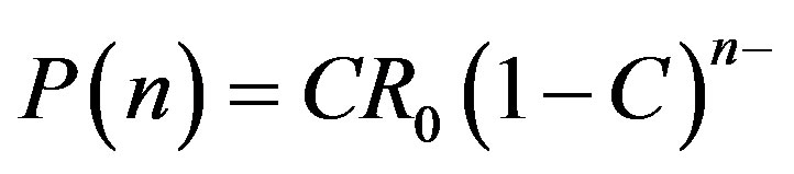 .
.
To do the proof, we need some additional elements of support:
Statement 1. By the definition of the Production Reserves Ratio, the reserves at successive years since the start of production are linked by the relationship: .
.
First it is established that Proposition 1.

where  represents the Reserves at year n, and R0 stands for the reserves at the beginning of the first year of production, or the Reserves at year zero, before production starts:
 .
.
Demonstration 1.
Theorem 1): For n = 1 the hypothesis of Proposition 1 is valid since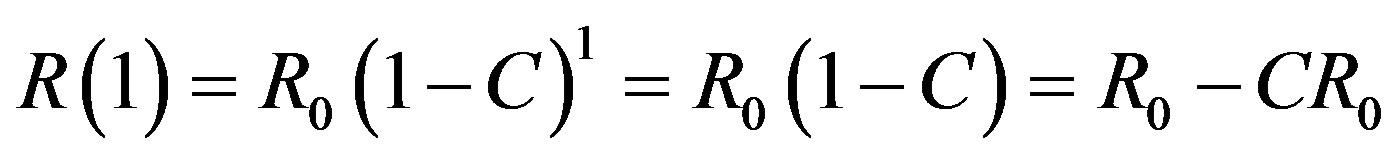 .
.
Theorem 2): Lets suppose the hypothesis is valid for n = m, what means: , where m is a natural number.
Lets show the hypothesis is valid for n = m + 1, that is .
.
That it is true since that from statement 1:
 .□
.□
Having demonstrated Theorems 1) and 2) we can rely on the principle of mathematical induction (Sominsky, 2000) to sustain .
.
Having demonstrated Proposition 1, the basis to support the Fundamental Equation requires the following developments:
Statement 2. By the law of conservation of matter, at year j the Production  equals the difference between the reserves at the end of the previous year minus the reserves at the end of the current year
 .□
.□
Statement 3. By Statement 1, Statement 2 means the Production  at the end of the current year j equals the multiplication of the production to reserves ratio C times the amount
  of reserves available at the end of the previous year, j − 1:
 , By Statement 1.
 .□
.□
With the support of the preceding results, lets proceed to demonstrate the fundamental equation of mineral production forecast: .
.
Theorem 1: For n = 1 the hypothesis is valid since .
.
Theorem 2: Lets suppose the hypothesis is valid for n = m, what means: , where m is a natural number.
Lets show the hypothesis is valid for n = m+1, that is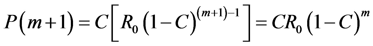 .
.
That it is true since by Statement 3: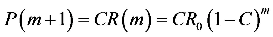 .
.
A detailed development of the above account is also available:
 .
.
Having demonstrated Theorems 1 and 2 we can rely on the principle of mathematical induction [22] to uphold
 .□
.□