Archaeological Discovery
Vol.03 No.02(2015), Article ID:55711,12 pages
10.4236/ad.2015.32008
Spot Reading of the Absolute Paleointensity of the Geomagnetic Field Obtained from Potsherds (Age Ca. 500-430 AD) in Teotihuacan, Mexico
Emilio Herrero-Bervera
Paleomagnetics and Petrofabrics Laboratory SOEST, Hawaii Institute of Geophysics and Planetology, University of Hawaii at Manoa, Honolulu, USA
Email: herrero@soest.hawaii.edu
Copyright © 2015 by author and Scientific Research Publishing Inc.
This work is licensed under the Creative Commons Attribution International License (CC BY).
http://creativecommons.org/licenses/by/4.0/


Received 20 February 2015; accepted 15 April 2015; published 16 April 2015
ABSTRACT
Archaeointensity data have been obtained successfully using the Thellier-Coe protocol from twelve potsherds recovered from the vicinity of the “Piramide del Sol”, Teotihuacan, Mexico. In order to understand the magnetic behavior of the samples, we have conducted low-field versus tempera- ture (k-T) experiments to determine the magnetic carriers of the pre-Columbian artefacts, as well as Saturation Isothermal Remanent Magnetization (SIRM), hysteresis loops and back-fields TESTS. The Curie temperatures indicate the presence of at least three magnetic mineral phases (238˚C - 276˚C, 569˚C - 592˚C, and 609˚C - 624˚C). The predominant Curie temperatures for these samples are typical of Ti-poor magnetite. The results of the magnetic grain size analyses indicate that if the magnetic mineral in a sample is only magnetite, the distribution on the modified Day et al. (1977) diagram yields specimens in the Single (SD), Pseudo (PSD) and Superparamagnetic (SP) domain ranges. The successfully absolute paleointensity determinations in this study using the Thellier-Coe protocol have yielded an average paleointensity of 38.871 +/− 1.833 m-Teslas (N = 12), and a virtual geomagnetic dipole moment of 8.682 +/− 0.402 × 10²² A/m2 which is slightly lower than the present field strength and which corresponds to an age interval between 500 and 430 AD. Thus, our results correlate well with the recently published CALS3K.4 curve and the incipient archaeointensity reference curve for the Mesoamerican paleo-field results. Therefore, the age of the artefacts would correlate well with absolute the early classic Teotihuacan cultural period.
Keywords:
Archaeointensity, Teotihuacan, Pottery Pieces

1. Introduction
It is well known that archeomagnetic determinations are important contributions to constraining the global and local variations of the Earth’s magnetic field in the recent past (e.g. present back to ~6000 years, e.g. Valet, Herrero-Bervera, LeMouël, & Plenier, 2008 ). Ideally, the best determinations are those for which the archaeomagnetic materials have been obtained from oriented artefacts that have rendered directional as well as absolute paleointensity results. In cases when it is not possible to experiment with oriented samples, the only possibility of obtaining an archeomagnetic observation is by means of the determination of the absolute paleointensity of the samples in question. Since the intensity of magnetization is a scalar quantity, it is not necessary to have the collected artefacts oriented. This allows one to experiment with a technique used for unique and single objects, such as pottery shards that have been found in their original firing position. In this way the absolute paleintensity method such as the Thellier-Coe protocol has been so far a more widely applicable technology (e.g. Genevey et al., 2008; Gallet et al., 2009 ; Alva-Valdivia et al., 2010). Archeological materials usually record events like the firing at some specific place and time; most archeomagnetic records are episodic both in space and time. Materials that are characterized by magnetic carriers such as iron oxides (e.g. magnetite, titanomagnetites and hematite) acquire a rather stable thermoremanent magnetization (i.e. a T.R.M.) whose direction is parallel to the Earth’s magnetic field at the time and place when the magnetic minerals cool through their Curie temperatures. Therefore, the magnetization of the archeomagnetic materials is proportional to the ambient field intensity. Thus, archeomagnetic studies of in situ structures such as pieces of pottery, ovens, kilns and hearths of dissimilar ages allow us to reconstruct the changes in direction and intensity of the Earth’s magnetic field for a given geographical region (e.g. Genevey & Gallet, 2002; Genevey et al., 2003, 2008 ). However, archeomagnetic materials that have been displaced from their original positions when they are originally fired i.e. in an unknown position, in most cases yield information only on the ancient geomagnetic field intensity (e.g. Stark et al., 2009 ). In this study we have undertaken absolute paleointensity determinations of un-oriented potshards from the Teotihuacan Pyramids close to Mexico City in order to determine the strength of the magnetic field of the Earth recorded at the last time of firing of the pieces of pottery under question.
2. Sampling
We have collected twenty seven pieces of un-oriented pottery from around the Pyramids of the Moon (see Figures 1(a)-(d)), the Sun and Plaza of the Moon (site latitude = 19.6925˚ North and longitude = 98.8438˚ West). Individual archaeomagnetic samples were prepared and cut to fit the 1 cm3 sample holder made of a non-mag- netic material (i.e. plexiglass) to treat them as standard paleomagnetic 1-cm3cores.
Measurements of remanences, archaeointensity (AI) determinations as well as Curie point determinations and magnetic granulometry analyses were performed using a JR5 Spinner magnetometer and a house made furnace with a Pyrox temperature controller housed in the magnetostatic shielded room, a low-field susceptibility vs. temperature (k-T) and a Variable Field Translation Balance (VFTB) instruments respectively of the SOEST- HIGP Petrofabrics and Paleomagnetics Laboratory of the University of Hawaii at Manoa.
3. Laboratory Experiments
3.1. Magnetic Mineralogy
Magnetic properties were analyzed to identify the magnetic carriers of the natural remanent magnetization (NRM) and to investigate the origin of the NRM. Studies of magnetic mineralogy were performed using 27 specimens of small pieces of fragments of pottery from the samples collected. Low-field susceptibility versus temperature (k-T) experiments were conducted in air using a magnetic anisotropy instrument MFK-1 with a CS-3 attachment in order to determine the Curie temperature of the samples. The specimens were progressively heated from room temperature up to 700˚C and subsequently cooled down using a CS-3 apparatus (Hrouda, 1994; Hrouda et al., 1997) . Several typical diagrams of susceptibility versus temperature (k-T) are shown in Figure 2. The Curie temperatures indicate the presence of at least three magnetic mineral phases (i.e. 238˚C - 276˚C, 569˚C - 592˚C, and 609˚C - 624˚C). The curves have very similar heating and cooling patterns. Both show predominantly the presence of the Curie temperature of magnetite. The presence of cation deficient (CD) magnetite was identified for some samples with Curie temperatures distributed in the range of 609˚C - 630˚C. It is interpreted that the apparent absence of hematite (Curie temperature 675˚C) may simply reflect its relative weak saturation magnetization,
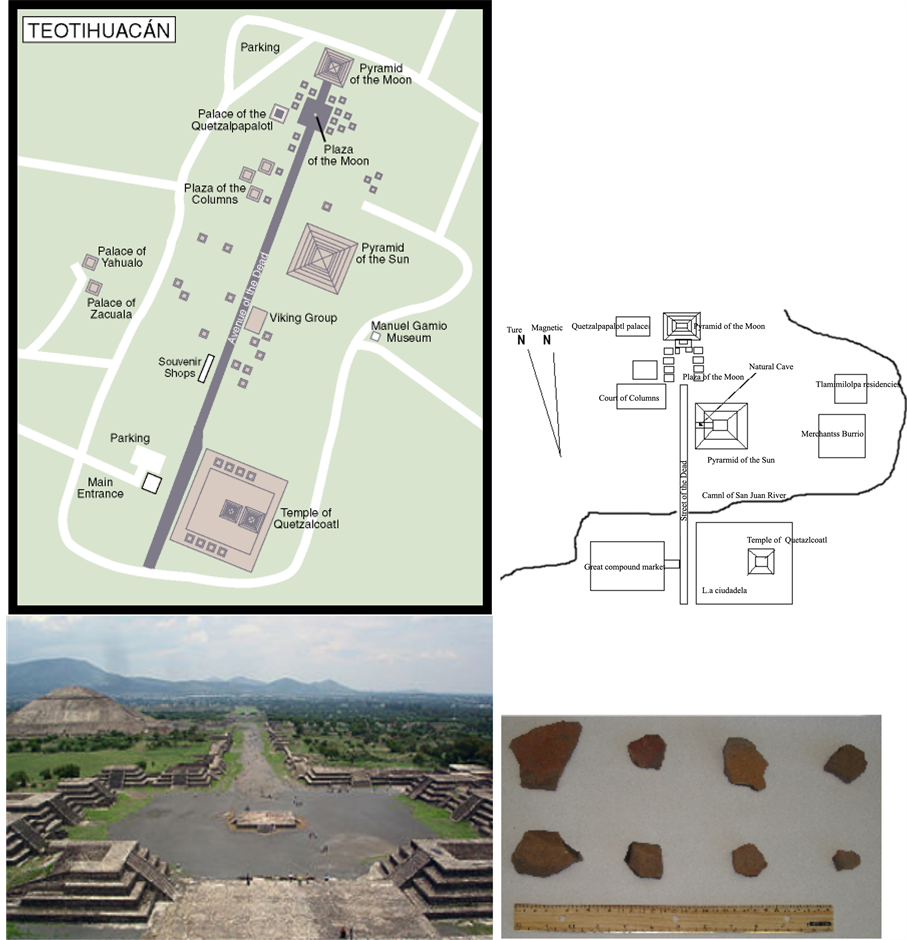
Figure 1. Location of the sampling sites. The upper left figure is a map of the Teotihuacan city close to Mexico City, where other potshards were collected from the surroundings of the Pyramids of Moon, the Sun and the Plaza of the Moon. The upper right a map of the same area showing the orientation of the site with respect to True and Magnetic North. The lower left corner picture shows a panoramic view of Teotihuacan. The lower right picture shows a set of eight pieces of pottery used for this study.
which is about two orders of magnitude less than that of magnetite. Therefore, when a significant portion of magnetite is present, the signal from hematite is swamped (e.g. Shaw et al., 1995 ). We have found out that most of the specimens studied had reversible heating and cooling results, with single inflection points, indicating Curie temperatures between 550˚C and 565˚C (see Figure 2, specimens 001, 003, 005, 008, 010, 016, and 022). We interpreted these data to indicate the predominance of low-Ti magnetite to pure magnetite as the primary magnetic minerals in these samples.
3.2. Magnetic Granulometry from Hysteresis Experiments
Magnetic hysteresis measurements were performed on the powder of ~200 mg from twenty seven potsherds us

Figure 2. Typical low-field susceptibility versus temperature (k-T) Curie point curves of 12 specimens from the Teotihuacan site. The red curve is the heating curve and the blue color represents the cooling curves. For the interpretation see text.
ing a variable field translation balance (VFTB) up to 1.2 T. Saturation remanent magnetization (Mr), saturation magnetization (Ms), and coercive force (Hc) were calculated after removing the paramagnetic contribution. We have determined the hysteresis loops and the back-field demagnetization curve of the saturation isothermal remanent magnetization (SIRM). The variable field translation balance (VFTB) instrument has a measuring range of 10−8 - 10−2 Am2. The coercivity of remanence (Hcr) suggests that the Isothermal Remanent Magnetization (IRM) is carried by low-coercivity grains. The ratios of the hysteresis parameters were plotted in Figure 3 as a modified Day diagram, following recent modifications by Dunlop (2002) for type curves and regions that have been defined for pure magnetite. Most grain sizes are scattered within the pseudo-single domain (PSD) range and few are also close to the superparamagnetic (SP) and single domain (SD) theoretical curves of Dunlop (2002) for the Teotihuacan potsherds (see Figure 3). It is striking that the distribution of coercivities is related to the unblocking temperatures. If we do not consider the influence of grain sizes, it is interesting to associate this distribution with the magnetic phases that are present in the sample. The hysteresis parameters have been initially defined from synthetic crystals of magnetite (Dunlop & Özdemir, 1997) . However we must point out that we are dealing with natural samples which contain magnetic grains associated with different mineralogical phases (see Figure 2). We speculate as to whether the characteristic values that separate the grain size domains for pure magnetite are entirely appropriate in the presence of several mineralogical components with overlapping coer-

Figure 3. Results of the hysteresis loops experiments performed on three representative samples of Teotihuacan potshards showing their diverse ratios of Mrs/Ms and Hcr/Hc parameters. The figure on the lower left shows hysteresis ratios for pottery samples compared to the theoretical Day plot curves calculated for magnetite using the equations developed by Dunlop (2002) . Detailed explanations of individual curves are given in Dunlop (2002) . Numbers along curves are volume fractions of the soft component (SP or MD) in mixtures with SD grains published by Dunlop (2002) .
civity spectra and magnetizations. This would probably explain why most studies deal with samples that are actually found within the pseudo-single domain range (e.g. Herrero-Bervera & Valet, 2009 ).
4. Paleointensity Experiments
Paleointensity experiments were conducted using the Coe version (Coe, 1967) of the Thellier and Thellier-ex- periments but with a different protocol. Instead of measuring the NRM first, we preferred to apply a TRM before heating the sample in zero field ( Aitken et al., 1988; Aitken, 1990 ; Valet et al., 1998; Herrero-Bervera & Valet, 2005, 2009; Herrero-Bervera & Acton, 2011 ). In this case, magnetomineralogical transformations occur in the presence of a field, resulting in a CRM (chemical remanent magnetization) component which is detected by a deviation of the NRM toward the oven field direction. Each heating step (beyond 100˚C and up to 540˚C) was accompanied by a pTRM check usually at the previous lower temperature step. The experiments were conducted in a Pyrox oven with a capacity of 80 samples. Heating control was carried out by three external thermocouples and accurate temperature control monitored by three additional thermocouples located close to the samples. Cooling was performed by sliding the heating chamber away from the hot specimens. Measurements were done using a JR-5 Spinner magnetometer (i.e. for the NRM, thermal demagnetization and for the absolute paleointensity measurements) in the shielded room of the SOEST-HIGP laboratory. Each series of experiments was carried out on 27 samples positioned a few millimeters away from each other within the oven. The magnetization level of the samples was too low to expect significant interactions between adjacent samples and effectively no remagnetization was observed in the demagnetization diagrams of the NRM, except those caused by subsequent magnetomineralogical transformations in the presence of a field.
Typical Arai plots are shown in Figure 4 and Figure 5 together with the evolution of the NRM during

Figure 4. Arai archaeointensity plot and evolution of NRM during thermal demagnetization for sample Teotihuacan-001. Notice the well defined linear NRM-TRM slope (from 100˚C up to 590˚C) and the positive pTRM checks (upper left corner diagram). Notice the remarkable tight clustering of the declination and inclination results depicted on the upper right corner of the diagram. The lower left represent the univectorial behavior of the directional results typical of the successful absolute paleointensity experiments. The lower right diagram are the results of the normalized intensity of magnetization indicating the predominance of one single magnetic mineral phase (e.g. Valet et al., 2010 ), in this case Ti-poor magnetite.

Figure 5. Six typical Arai plots for Teotihuacan specimens. Black squares represent the initial NRM-pTRM measurements, open squares are NRM-pTRM checks. Rejection was decided on the basis of the deviation of the pTRM checks following the criteria that have been put forward in the present study (see text). Diagrams without linear NRM-pTRM segments were rejected and thus not shown here.
thermal demagnetization. The paleointensity results have been summarized in Table 1 for the 12 potsherds that yielded successful AI determinations. We have selected Arai diagrams with various configurations. The samples from the Teotihuacan potshards exhibit a linear slope over the same range of unblocking temperatures as those that were used to define the characteristic direction of magnetization. This illustrates the importance of considering the entire vector in the interpretation of the Arai diagram. In a number of cases some pTRM checks deviate slightly, but not very significantly, from the original TRM and must thus be considered as marginally negative. This is the case for a few samples which exhibit at least two negative checks. In some other specimens (e.g. sample Teo-026) only one pTRM check is slightly negative. In all cases, it is striking that all datapoints define anexcellent linear NRM-TRM segment over the entire temperature spectrum that is associated with the decay of the NRM. Apart from these small deviations of the checks, there would be no major reason to rule out such samples and there is no ambiguity regarding the determination of its NRM-TRM slope. For the samples with positive pTRM checks,the magnetic mineralogy is dominated by magnetite with a narrow range of high unblocking temperatures (see Figure 2 and Figure 4). Note that these determinations point out the importance of performing pTRM checks at all steps of the experiment. Because this has rarely been the case, it could be one additional factor that generates dispersion.
As mentioned above, the large deviations observed in some rejected samples are characterized different

Table 1. Sample number indicates the Teotihuacan specimens used for the statistical analyses, Tre (oC) is the temperature interval involved in the calculation of the paleofield, N is the number of data points (N points) involved in the calculation of the slope and their dispersion (S.D.). Paleo H is the obtained paleofield in μT. Q, w, f, w are the quality factor, the weight factor, the NRM fraction of the linear TRM-NRM portion that has been considered for calculation of paleointensity and the gap factor, respectively. Hlab is the applied field in the laboratory experiments, Slope of the linear fit and the sigma error of the slope.
magnetic phases such as titanomagnetite and/or some maghemite (i.e. other minerals than pure magnetite). The relative proportion of single domain magnetite with high blocking temperatures can be roughly estimated by the amount of magnetization remaining above temperatures exceeding 400˚ - 500˚C (e.g. Herrero-Bervera & Valet, 2009 ). There is a clear relationship between the complexity of the mineralogy and the fidelity of the paleointensity experiment for the Teotihuacan samples. It is important to point out that this magnetic mineralogy characteristic is consistent with the large success rate of the archeointensity studies because the magnetization of the archeomagnetic materials is mostly dominated by a unique mineral such as Ti-poor magnetite (e.g. Valet et al., 2010 ) which is the case of the twelve successful Teotihuacan samples of this study (see Figure 4 and Figure 5).
5. Discussion and Conclusion
So far, various methods have been suggested to select the appropriate data for absolute paleointensity interpretation (PI) of the results despite the fact that much debate questions what constitutes acceptable PI determinations. In the best of cases, it is necessary for the samples in question to have reversible Curie point determination curves, which in a certain way give evidence that no apparent magnetomineralogical changes/alterations have occurred during the laboratory heating procedure, and for samples to be characterized by either single domain or an admixture of Pseudo Single and Single Domains (PSD/SD) magnetic grain sizes. As it can be observed from the magnetic grain sizes diagram of Figure 3, the great majority of the Teotihuacan sepcimens are in the PSD and close to the Super Paramagnetic (SP) theoretical envelope of Dunlop (2002) , and also very few samples are situated around the SD-Multidomain (MD) area.
For the successful Teotihuacan pieces of pottery, we have followed three fundamental criteria here. 1) The characteristic (primary) remanent magnetization component must decay to the origin of a vector demagnetization diagram (e.g. see univectorial demagnetization diagram of Figure 4); 2) the slope of the line in Arai plots must be linear over the temperature range where the primary Thermo-Remanent Magnetization (TRM) is resolved; 3) the partial TRM (pTRM) checks must not deviate significantly from the TRM on sequential temperature steps (e.g. see Figure 4 and Figure 5).
The first criterion is used in various forms in current paleointensity studies (e.g., Perrin, Schnepp, & Shcherbakov, 1998; Zhu et al., 2001 ). Each deviation from the demagnetization path from the origin of vector demagnetization diagrams introduces a significant uncertainty in the determination of paleointensity, as it reflects failure to isolate the primary TRM. When plotted in sample coordinates, the evolution of the NRM direction also gives crucial information about possible deviations caused by CRMs that have higher unblocking temperatures than the last heating step. Samples that exhibit remagnetization during heating in the presence of the field are characterized by large directional swings of the remaining NRM towards the direction of the applied field. In the present study this was the case for 15 samples rejected for the analyses of the AI study. This criterion is probably particularly effective as a consequence of our protocol that requires that laboratory TRM acquisition precede demagnetization in zero field. The demagnetization diagrams are also important for determining the temperature range over which the primary TRM has been isolated. Samples in which a significant part of the stable TRM is carried by SD grains of magnetite generally are less affected by large viscous components, low-temperature overprints, or other sources of overprints. In such cases, a significant percentage of the total NRM intensity remains after removing any viscous components or overprints, allowing the primary TRM to be resolved along linear demagnetization paths that trend to the origin of vector demagnetization diagrams and allowing the viscous or over printed temperature range to be avoided in Arai plots.
The second criterion retains only Arai plots with a single linear slope within the temperature range that lie above the viscous domain. We have required that the fit of the line must be better than R = 0.98 as depicted in the Arai plots of Figure 5 for the twelve successful paleointensity determinations. Due to our selection rules, the averaged number of points used for slope determination amounts to 10 and never less than 7 and the “f” (NRM fraction of Coe et al., 1978 ) parameters are always greater than 75% percent (see Table 1). In our case the range of the “f” parameter is from 75.5 up to 97. It is important to point out that this parameter is meaningless when there is a strong viscous low temperature component with an opposite direction to the characteristic remanence, which is not the case for the 12 samples in question and when the average quality factor lies much beyond the limits of1 or 2 that are usually required. In the case of the Teotihuacan samples the quality factor ranges between 7.7 up to 33 (see Table 1). The mean value of the gap ratio (see Table 1, gap factor of Coe et al., 1978 ) measuring the relative uncertainty on the definition of the best-fit line is almost twice weaker than the acceptable limit of 0.1 (see Selkin & Tauxe, 2000 ); the range of the gap factor is from 0.63 up to 0.85 for this study.
The third criterion rejects the results if the pTRM checks were consistently negative: that is they differ significantly from the initial TRM on several sequential temperature steps. Different investigators use different cutoff values for what they consider significant, and often base their rejection on single pTRM checks. Here, pTRM checks were considered to be negative when they deviated by more than 5% from the initial TRM, and they did so on sequential temperature steps. We believe that such cutoffs applied to single temperature steps are somewhat arbitrary when pTRM checks are performed systematically after nearly every heating step. Indeed, small deviations of the pTRM checks from the initial TRM can be caused by mineralogical transformations or by experimental uncertainties. In the first case, the subsequent thermal steps will typically be systematically accompanied by progressively larger deviations, which confirm that the sample must be rejected. In the second case, subsequent checks will not be negative and hence a reliable paleointensity determination may be obtained over the temperature interval. Generally, samples that failed the second or third criterion had already notably failed the first criterion, which was the most effective data selection criterion.
Out of the 27 absolute paleointensity experiments, only twelve specimens from the Teotihuacan collection gave acceptable PI results. Arai plots, low-field susceptibility versus temperature (k-T) Curie point determinations and vector demagnetization diagrams shown in Figures 3-5 for the samples in question and the summarized PI results given in Table 1 attest for the best results of the experiments we have conducted on the potshards from Teotihuacan.
The main goal of this study is to determine the strength of the Earth’s magnetic field recorded by the pieces of pottery recovered from the Teotihuacan Pyramids. This goal has been achieved and the estimated average archaeomagnetic absolute paleointensities after a correction for the dependency of the TRM with the cooling rate (e.g. Chauvin, 2000; Tema et al., 2012; Aguilar Reyes et al., 2013; Alva-Valdivia et al., 2010; Fanjat et al., 2013 ) obtained in this study is 38.871 +/− 1.833 m-Teslas (N = 12), and a virtual geomagnetic dipole moment of 8.682 +/− 0.402 × 10²² A/m2 which is slightly lower than the present field strength.
The second goal of this study is to correlate the AI results with the master curves and models available for the central part of Mesoamerica since, this study so far does not have a 14C radiometric age determined using the potshards in question. I have tentatively done a correlation with the CALS3K.4 curves for the past 3 ka (Donadini et al., 2009; Korte & Constable, 2011; Korte, Constable, Donadini, & Holme, 2011) and the Mesoamerica curves of the studies published by Aguirre et al. (2013) and Alva-Valdivia et al. (2010) . The selected spot reading of the paleofield agrees reasonably well to an age interval between 500 and 430 AD, (“present” = AD 1950), see Figure 6. The implication of this AI determination correlation to the Aguirre et al. (2013) study indicates that the potshards were made during the early classic cultural period and the oxygen isotope record corresponding to drier times in Teotihuacan, see Figure 7. These last interpretations and the oxygen isotope record have to be taken with caution since this study does not have a direct 14C radiometric age determination of the potshards used for the present study. The AI determination of this study has also been plotted up using the GEOMAGIA 50 published by Korhonen et al. (2008) as depicted in Figure 8.

Figure 6. Time variation of Archaeo-Intensity (AI) data (triangles) plotted together with ArcheoInt database. Continuous brown (blue) line represents a correlation with the model ARCH3k (CALS3k). Also shown Cuanalan and Xitle latest AI determination. The red open circle represents the AI result of this study. The figure is taken and modified from Alva-Valdivia et al. (2010) .

Figure 7. (a) Currently available absolute intensity data from Mesoamerica derived from archeological artifacts and historic lava flows (Aguilar et al., 2013). Also shown are the data derived from model prediction from CALS3K.4 for the past 3 ka and CALS10K.1b for the past 10 ka. (b) Oxygen isotope record from Punta Laguna, northern Yucatan lake, Mexico. (c) Major societal changes in Mesoamerica. All the data are drawn versus calendar age and Maya cultural periods. The figure is taken and modified from Aguilar et al. (2013). The blue open circle represents the AI result obtained from this study.

Figure 8. Archaeointensity Mexican data from GEOMAGIA v.2 database from Korhonen et al., 2008. The top diagram represents Age (years) versus Virtual Axial Dipole Moment (VADM, 1022 Am2) and the lower plot is Age (years) versus Paleointensity in m-Teslas. The red rhombs represent the absolute paleointensity determinations obtained from this study. The error bars are within the red rhombs. The black dots are reduced to central Mexico (Site Latitude = 19.6925˚North and Longitude = 98.8438˚West).
Acknowledgements
I gratefully acknowledge the assistance of Mr. James Lau during the laboratory phase of this project and Mrs. N. Herrero for the assistance during the sample collection at the Teotihuacan Pyramids. Thanks to Dr. Evdokia Tema for her help with the GEOMAGIA plots. We also thank two anonymous reviewers for their very constructive criticisms. Funding for this research was provided by SOEST-HIGP of the University of Hawaii at Manoa. This a SOEST contribution # 9295 and HIGP # 2065.
References
- Aguilar Reyes, B., Goguitchaichvili, A., Morales, J., Gardun˜o, V. H., Pineda, M., Carvallo, C., Moran, T. G., Israde, I., & Rathert, M. C. (2013). An Integrated Archeomagnetic and C14 Study on Pre-Columbian Potsherds and Associated Charcoals Intercalated between Holocene Lacustrine Sediments in Western Mexico: Geomagnetic Implications. Journal of Geophysical Research: Solid Earth, 118, 2753-2763. http://dx.doi.org/10.1002/jgrb.50196
- Aitken, M. J. (1990). Science-Based Dating in Archaeology (pp. 225-229). Longman Archaeology Series, London and New York: Longman.
- Aitken, M. J., Allsop, A. L., Bussell, G. D., & Winter, M. B. (1988). Determination of the Intensity of the Earth’s Magnetic during Archaeological Times: Reliability of the Thellier Technique. Reviews of Geophysics, 26, 3-12. http://dx.doi.org/10.1029/RG026i001p00003
- Alva-Valdivia, L. M., Morales, J., Goguitchaichvili, A., Popenoe de Hatch, M., Hernandez-Bernal, M. S., & Mariano-Matías, F. (2010). Absolute Geomagnetic Intensity Data from Preclassic Guatemalan Pottery. Physics of the Earth and Planetary Interiors, 180, 41-51. http://dx.doi.org/10.1016/j.pepi.2010.03.002
- Chauvin, A., Garcia, Y., Lanos, Ph., & Laubenheimer, F. (2000). Paleointensity of the Geomagnetic Field Recovered on Archaeomagnetic Sites from France. Physics of the Earth and Planetary Interiors, 120, 111-136. http://dx.doi.org/10.1016/S0031-9201(00)00148-5
- Coe, R. S. (1967). Paleo-Intensities of the Earth’s Magnetic Field Determined from Tertiary and Quaternary Rocks. Journal of Geophysical Research, 72, 3247-3262. http://dx.doi.org/10.1029/JZ072i012p03247
- Coe, R. S., Grommé, S., & Mankinen, E.A. (1978). Geomagnetic Paleointensities from Radiocarbon-Dated Lava Flows on Hawaii and the Question of the Pacific Nondipole Low. Journal of Geophysical Research: Solid Earth, 83, 1740-1756. http://dx.doi.org/10.1029/JB083iB04p01740
- Day, R., Fuller, M., & Schmidt, V. A. (1977). Hysteresis Properties of Titanomagnetites: Grain Size and Composition Dependence. Physics of the Earth and Planetary Interiors, 13, 260-267. http://dx.doi.org/10.1016/0031-9201(77)90108-X
- Donadini, F., Korte, M., & Constable, C. G. (2009). Geomagnetic Field for 0 - 3 ka: 1. New Data Sets for Global Modeling. Geochemistry, Geophysics, Geosystems, 10, pp. http://dx.doi.org/10.1029/2008GC002295
- Dunlop, D. J. (2002). Theory and Application of the Day Plot (Mrs/Ms versus Hcr/Hc) 2. Application to Data for Rocks, Sediments and Soils. Journal of Geophysical Research, 107, EPM5-1-EPM5-15.
- Dunlop, D. J., & Özdemir, O. (1997). Rock Magnetism: Fundamentals and Frontiers (573 p.). New York: Cambridge University Press. http://dx.doi.org/10.1017/CBO9780511612794
- Fanjat, G., Camps, P., Alva Valdivia, L. M., Sougrati, M. T., Cuevas-Garcia, M., & Perrin, M. (2013). First Archeointensity Determinations on Maya Incense Burners from Palenque Temples, Mexico: New Data to Constrain the Mesoamerica Secular Variation Curve. Earth and Planetary Science Letters, 363, 168-180. http://dx.doi.org/10.1016/j.epsl.2012.12.035
- Gallet, Y., Genevey, A., Le Goff, M., Warmé, N., Gran-Amorich, J., & Lefevre, A. (2009). On the Use of Archeology in Geomagnetism, and Vice-Versa: Recent Developments in Archeomagnetism. Comptes Rendus Physique, 10, 630-648. http://dx.doi.org/10.1016/j.crhy.2009.08.005
- Genevey, A. S., Gallet, Y., & Margueron, J. C. (2003). Eight Thousand Years of Geomagnetic Field Intensity Variations in the Eastern Mediterranean. Journal of Geophysical Research, 108, NIL20-NIL37. http://dx.doi.org/10.1029/2001JB001612
- Genevey, A., & Gallet, Y. (2002). Intensity of the Geomagnetic Field in Western Europe over the Past 2000 Years: New Data from Ancient French Pottery. Journal of Geophysical Research, 107, EPM1-1-EPM1-18. http://dx.doi.org/10.1029/2001JB000701
- Genevey, A., Gallet, Y., Constable, C. G., Korte, M., & Hulot, G. (2008). ArcheoInt: An Upgraded Compilation of Geomagnetic Field Intensity Data for the Past Ten Millennia and Its Application to the Recovery of the Past Dipole Moment. Geochemistry, Geophysics, Geosystems, 9, Q04038. http://dx.doi.org/10.1029/2007GC001881
- Herrero-Bervera, E., & Acton, G. (2011). Absolute Paleointensities from an Intact Section of Oceanic Crust Cored at ODP/IODP Site 1256 in the Equatorial Pacific. In E. Petrovsky, D. Ivers, T. Harinarayana, & E. Herrero-Bervera (Eds.), The Earth’s Magnetic Interior, IAGA Special Sopron Book Series 1 (pp. 181-193). Berlin: Springer Science + Business Media B.V.
- Herrero-Bervera, E., & Valet, J. P. (2009). Testing Determinations of Absolute Paleointensity from the 1955 and 1960 Hawaiian Flows. Earth and Planetary Science Letters, 287, 420-433. http://dx.doi.org/10.1016/j.epsl.2009.08.035
- Herrero-Bervera, E., &Valet, J. P. (2005). Absolute Paleointensity and Reversal Records from the Waianae Sequence (Oahu, Hawaii, USA). Earth and Planetary Science Letters, 234, 279-296. http://dx.doi.org/10.1016/j.epsl.2005.02.032
- Hrouda, F. (1994). A Technique for the Measurement of Thermal Changes of Magnetic Susceptibility of Weakly Magnetic Rocks by the CS-2 Apparatus and KLY-2 Kappabridge. Geophysical Journal International, 118, 604-612. http://dx.doi.org/10.1111/j.1365-246X.1994.tb03987.x
- Hrouda, F., Jelinek, V., & Zapletal, K. (1997). Refined Technique for Susceptibility Resolution into Ferromagnetic and Paramagnetic Components Based on Susceptibility Temperature Variation Measurements. Geophysical Journal International, 129, 715-719. http://dx.doi.org/10.1111/j.1365-246X.1997.tb04506.x
- Korhonen, K., Donadini, F., Riisager, P., & Pesonen, L. (2008). GEOMAGIA50: An Archeointensity Database with PHP and MySQL. Geochemistry, Geophysics, Geosystems, 9, 893.
- Korte, M., & Constable, C. G. (2011). Improving Geomagnetic Field Reconstructions for 0 - 3 ka. Physics of the Earth and Planetary Interiors, 188, 247-259. http://dx.doi.org/10.1016/j.pepi.2011.06.017
- Korte, M., Constable, C. G., Donadini, F., & Holme, R. (2011). Reconstructing the Holocene Geomagnetic Field. Earth and Planetary Science Letters, 312, 497-505. http://dx.doi.org/10.1016/j.epsl.2011.10.031
- Perrin, M., Schnepp, E., & Shcherbakov, V. (1998). Paleointensity Database Updated. Eos, Transactions American Geophysical Union, 79, 198. http://dx.doi.org/10.1029/98EO00145
- Selkin, P., & Tauxe, L. (2000). Long-Term Variations in Paleointensity. Philosophical Transactions of the Royal Society A, 358, 1065-1088. http://dx.doi.org/10.1098/rsta.2000.0574
- Shaw, J., Yang, S., & Wei, Q. Y. (1995). Archaeointensity Variations for the Past 7,500 Years Evaluated from Ancient Chinese Ceramics. Journal of Geomagnetism and Geoelectricity, 47, 59-70. http://dx.doi.org/10.5636/jgg.47.59
- Stark, F., Leonhardt, R., Fassbibder, J. W. E., & Reindel, M. (2009). The Field of Sherds: Reconstructing Geomagnetic Field Variations from Peruvian Potsherds. In M. Reindel, & G. A. Wagner (Eds.), New Technologies for Archaeology, Natural Science in Archaeology (pp. 103-116). Berlin: Springer-Verlag.
- Tema, E., Gomez-Pacard, M., Kondopoulou, D., & Almar, Y. (2012). Intensity of the Earth’s Magnetic Field in Greece during the Last Five Millennia: New Data from Greek Pottery. Physics of the Earth and Planetary Interiors, 202-203, 14-26. http://dx.doi.org/10.1016/j.pepi.2012.01.012
- Valet, J. P., Herrero-Bervera, E., Carlut, J., & Kondopoulou, D. (2010). A Selective Procedure for Absolute Paleointensity in Lava Flows. Geophysical Research Letters, 37, L16308. http://dx.doi.org/10.1029/2010GL044100
- Valet, J. P., Herrero-Bervera, E., LeMouël, J. L., & Plenier, G. (2008). Secular Variation of the Geomagnetic Dipole during the Past 2000 Years. Geochemistry, Geophysics, Geosystems, 9, Q01008.
- Zhu, R., Pan, Y., Shaw, J., Li, D., & Li, Q. (2001). Geomagnetic Palaeointensity just Prior to the Cretaceous Normal Superchron. Physics of the Earth and Planetary Interiors, 128, 207-222. http://dx.doi.org/10.1016/S0031-9201(01)00287-4