American Journal of Computational Mathematics
Vol.07 No.03(2017), Article ID:78151,15 pages
10.4236/ajcm.2017.73020
Random Timestepping Algorithm with Exponential Distribution for Pricing Various Structures of One-Sided Barrier Options
Hasan Alzubaidi
Department of Mathematics, Al-Qunfudah University College, Umm Al-Qura University, Mecca, KSA

Copyright © 2017 by author and Scientific Research Publishing Inc.
This work is licensed under the Creative Commons Attribution International License (CC BY 4.0).
http://creativecommons.org/licenses/by/4.0/


Received: Jun 29, 2017; Accepted: July 31, 2017; Published: August 3, 2017
ABSTRACT
The exponentially-distributed random timestepping algorithm with boundary test is implemented to evaluate the prices of some variety of single one-sided barrier option contracts within the framework of Black-Scholes model, giving efficient estimation of their hitting times. It is numerically shown that this algorithm, as for the Brownian bridge technique, can improve the rate of weak convergence from order one-half for the standard Monte Carlo to order 1. The exponential timestepping algorithm, however, displays better results, for a given amount of CPU time, than the Brownian bridge technique as the step size becomes larger or the volatility grows up. This is due to the features of the exponential distribution which is more strongly peaked near the origin and has a higher kurtosis compared to the normal distribution, giving more stability of the exponential timestepping algorithm at large time steps and high levels of volatility.
Keywords:
Barrier Option with Rebate Payment, Binary Barrier Option, Partial Barrier Option, Hitting Time Error, Exponential Time-Stepping Algorithm

1. Introduction
Barrier options are path-dependent exotic options with payoff depending on the price of the underlying asset at expiration and whether or not the asset price reaches a pre-specified barrier during the option’s life [1] . Since 1976, barrier options have become extremely popular and have been traded in the over-the counter (OTC) market. There are two main types of such options: knock-in (up-and-in and down-and-in) and knock-out (up-and-out and down-and-out) that can either have put or call feature. The up and down refer to the position of the barrier relative to the initial asset price. The in and out specify the type of the barrier, referring to activating and inactivating when the barrier is hit, respe- ctively. In 1973, Merton [2] derived the first analytical formula for the down- and-out call option. In 1991, Reiner and Rubinstein [3] extended this work further to provide closed form solutions for all eight types of single barrier options in Black-Scholes environment. Later in 1998, Haug [4] gave a generalization of these formulas in order to complete the total sixteen pricing formulae for the barrier options.
Some barrier options specify that a fixed cash rebate is to be given to the option-holder if the knock-out and knock-in options become worthless. This can make the barrier options more attractive to the potential purchasers by compensating them for the loss of the option when the knock-out option ceases to exist or when knock-in option comes into existence [5] . The valuation of such an option can be then expressed as the sum of the payoff of the standard barrier option with zero rebate and the payoff of the pure rebate option [6] .
However, the rebate options are not necessarily be combined with the standard barrier options and in this case the rebate options are usually called binary or digital barrier options [6] . These options can be divided into two main types: cash-or-nothing barrier options and asset-or-nothing barrier options. The payoff of the cash-or-nothing option is either a fixed amount of money or nothing at all, depending on whether the asset price has crossed the given barrier or not. For the asset-or-nothing barrier option, the payoff is the value of the underlying asset or nothing at all, depending on whether the asset price has crossed the given barrier or not [4] . These options are widely traded in the OTC market as hedges against jump risk and in the sports betting industry, due to the binary in nature of their payoffs [7] . They are also important for financial engineers as building blocks for constructing more complex derivatives products [4] . In 1991, Reiner and Rubinstein derived analytical formulas for pricing 28 different types of knock-out and knock-in call or put binary barrier options in Black-Scholes enviroment [3] [4] .
Since early nineties, more complicated structures of barrier options have been innovated according to clients and investors needs. For controlling starting and ending time of the monitoring period, one can use partial-time barrier option, where the underlying price is monitored during a fraction of the option’s lifetime [4] . Heynen and Kat (1994) gave closed form valuation formulae for pricing this type of options in terms of bivariate normal distribution functions [4] [8] . Partial-time barrier options have two main types: early-ending and forward- starting barrier options. The first one is known as type A partial-time barrier option where the monitoring period of the barrier starts at the option’s initial starting date and ends early at some time before expiration. The other is called type B partial-time barrier option where the barrier option becomes active at an arbitrary time before expiration and ends at maturity date [4] .
The analytical expressions for the barrier options, however, are available only under these particular frameworks and in fact, many other cases such as options with multiple assets and some path-dependent options have not explicit formulae yet. Therefore, accurate numerical and Monte Carlo simulation procedures play crucial role in this situation.
Barrier options are considered as exit time problems and therefore large errors can occur when direct Monte Carlo simulations are used. Specifically, Monte Carlo algorithm for pricing the continuously monitored barrier options has slow convergence and produces high statistical and hitting time errors, due to the knockout feature of such options [9] . We here concentrate on analyzing the hitting time error and how to reduce it efficiently. In fact, the direct MC simulation overestimates the actual values of the barrier option prices due to the possibility that these prices may hit the barrier and comeback within the time step, say , producing a hitting time error with order of convergence of [9] .
A clever idea to reduce this kind of error efficiently is to apply a simple hitting test after each time step using the distribution of the Brownian bridge pinned between the discrete computational nodes, in order to check if the barrier is crossed during the time step or not [9] [10] . This technique is known as a Brownian bridge technique and according to Gobet [11] , using this simple technique can improve the order of convergence from to under some conditions on functional of the asset price. For more analysis on using the Brownian bridge technique, see for example [9] - [16] and the refer- ences quoted therein.
In this paper, we present an analogous method called the exponential timestepping algorithm introduced by Jansons and Lythe [17] [18] for simulating the hitting time of one-dimensional diffusion models. Under this technique, in place of a fixed time step , we take time steps that are i.i.d exponentially distributed random variables and , where the rate plays the role of discretization parameter. The random
time step then has the expectation as equivalent to the fixed
time step . Analogously to the Brownian bridge technique, the probability that the barrier has been hit during the time step can also be taken into account using an efficient boundary hitting test at the end of each time step. Numerical experiments for the double-well potential physical problem [18] and for the neural diffusion models [12] show that incorporating this boundary test with exponential timestepping can retrieve a first order of convergence in approximating hitting time, coinciding with our numerical observations for financial derivatives of barrier feature. Although, in general, both techniques achieve similar levels of accuracy, the random timestepping method, in simulating hitting time, gives better results than the fixed timestepping method at large time steps and high levels of volatility, due to the features of the exponential distribution. This distribution has a memoryless property and is highly peaked near the origin, compared to the Gaussian distribution [19] . The distribution of the diffusion process at the end of the exponential time step , conditional on it having hit the given barrier during the time step, is the same as if the time step had started at the barrier [17] [18] . The price to be paid is uncertainty since the precise value of the time step is not formally known,
but its mean value is given as . The total elapsed time after time steps is thus a random variable with mean [18] .
The contribution of this work is to present an efficient method for simulating the exit time or functional of the exit time of one dimensional diffusion models such as barrier options in environment of Black-Scholes models. The remainder of this paper is structured as follows. Section 2 discuses the analytical expre- ssions for valuating some variety of one-sided barrier options contracts in Black- Scholes environment. In Section 3, we describe the implementation of the exponential timestepping algorithm with boundary test for pricing the three types of one-sided single barrier options outlined in the previous section. Section 4 includes our numerical experiments concerning these barrier options, in order to compare such an algorithm for efficiency and accuracy with the well-known algorithm called the Brownian bridge technique. The hitting time errors are also discussed and analyzed. Section 5 presents our concluding remarks and some ideas for future work.
2. Valuation of Barrier Options
We here consider some of different structures of one-sided barrier options within the framework of Black-Scholes model. Thus, under a risk-neutral measure the asset price is represented by a geometric Brownian model:
(1)
where is a standard Brownian motion and is the constant volatility of the asset price. , is the drift under the risk-neutral probability, where and represent the risk-free interest rate and the continuous dividend payable, respectively. The first hitting time of the asset price with barrier , where and is expiry time, is thus defined by
(2)
Based on above, we will discuss the valuation of some variety of one-sided barrier option contracts in the Black-Scholes environment as follows.
2.1. Vanilla Barrier Options with Pre-Specified Cash Rebate
As a case study, we consider up-and-out put vanilla barrier option with cash rebate and other forms can be dealt with, in the same manner. The discounted payoff of such an option at risk-free interest rate is given by [4]
(3)
The value of the option price at time can be formally given as [4]
(4)
where the expectation here is taken with respect to the risk-neutral probability measure , is rebate payment and is strike price of the barrier option.
The theoretical value of such an option can be calculated as the sum of the values of the up-and-out put option with zero rebate and a pure rebate
option . To calculate , we first consider , , and , where and represent the volatility and dividend payable respectively. The value of the up-and-out put option with zero rebate is thus given by [4] [6]
(5)
where
denotes the standard normal distribution function defined as
The pure rebate option can be calculated as [4] [6]
(6)
Consequently, the up-and-out put option with cash rebate can be given as
(7)
2.2. Binary Barrier Options
Here, we consider the down-and-out cash-or-nothing option as an example of binary barrier options. The holder of this contract will receive a fixed cash amount only if the underlying asset price never hits the barrier from above before the expiry date . Otherwise, the option will expire without value. The discounted payoff of such an option with at risk-free interest rate is given by [6]
(8)
The value of the down-and-out cash-or-nothing option price at time can be formally given as [4]
(9)
where the expectation here is taken with respect to the risk-neutral probability measure and is pre-specified cash amount.
The theoretical value of the down-and-out cash-or-nothing option at time with barrier , can be calculated as [4] [6] [7]
(10)
where . , and are defined as above.
2.3. Partial-Time Single-Asset Barrier Options
The type A (early-ending) partial-time barrier option is considered here as an example of partial-time single-asset barrier options. This type of option is defined such that the barrier starts at time and ends at some time . Since the barrier will end before the expiration time , we do not need to distinguish whether or . Therefore, we have a total of eight varieties of type A partial-time barrier option. As an example, we discuss a down-and-out call partial-time barrier option, where the option is knocked out during the interval as soon as the underlying price is below the barrier . The discounted expected payoff for such an option at risk-free interest rate can be thus written as: [8]
(11)
The value of the down-and-out call partial-time barrier option at time can be formally given as [4]
(12)
where the expectation here is taken with respect to the risk-neutral probability measure .
The closed form formula for pricing this type of options was originally derived by Heynen and Kat as [4] [8]
(13)
where , , , , , , , , , and is bivariate normal distribution.
3. Exponential Timestepping Algorithm with Boundary Test
The strategy of this algorithm is based on approximating the asset price of the underlying barrier option at each time by a Brownian motion with a constant drift , , where and are constants, with parameters determined at the current position and in this case, the increment has a symmetric exponential distribution [18] . Thus, exact calculations can be easily obtained for the density of and the probability that the barrier being hit during the exponential time step. We then update the exponential timestepping method for using these calculations. First, the density of can be written as
(14)
where and . Integrating over the density of defined in Equation (14) yields
(15)
and thus has exponential distribution and can be easily sampled. To produce updates for using these calculations, we first consider a uniformly distributed random variable in and an exponentially distributed random variable that can be generated as , where and is independent of . Then with given the value , we generate the value of for , where is exponential time step
with , as [18]
(16)
where and . where the quantity comes from Equation (15) by setting .
Next, a simple posteriori test is performed after each time step in order to calculate the conditional probability of a given barrier being hit during the time step [18] . This probability can be calculated as [18]
(17)
and
(18)
Then, an excursion is deduced in if
for the case of up barrier options and
for down barrier options, where is a uniformly distributed random variable. The time stepping will be repeated until this hitting event is detected or the maximum number of exponential time steps is reached. The output is hitting
time approximated as , where is the number of taken time steps. Based
on this, the discounted payoffs of the three cases of the underlying barrier options discussed in Section 2 are calculated using (3), (8) and (11), respectively. The prices of the underlying barrier options are then computed as the expectations of such discounted payoffs under the risk-neutral measure. A monte Carlo procedure is therefore used to estimate these expectations by a sample average of independent simulations; see Appendix A for full algorithm.
4. Summary of Numerical Results
In our numerical experiments, the mean value of the random time step
is used in the exponential timestepping algorithm as equivalent to the fixed time step in the Brownian bridge technique. We employ these simulation algorithms for the three types of one-sided single barrier options outlined in Section 2, and compare the efficiency of such techniques. The hitting time errors will be discussed and analyzed.
For the first type, we consider up-and-out put vanilla barrier option with rebate payment, and its computational results are displayed in Figure 1 and Table 1. The plots of the hitting time error calculated using the two underlying
simulation techniques against the discretization parameter are shown
in log-log scale at the top of Figure 1, and the plots of the CPU time as a function of hitting time error are shown at the bottom of the figure. The parameters are fixed as the volatility parameter , the dividend , the risk-free interest rate , the current value of the option

Table 1. Hitting time errors and standard errors for the up and out put barrier option with rebate payments with , .

Figure 1. (a) Plots of the hitting time error calculated using the Brownian bridge technique and the exponential time stepping algorithm against the discretization parameter for the up and out put barrier option with rebate payments. The parameters are fixed as: the volatility parameter , the dividend , the risk-free interest rate , the current value of the option , the strike price , the barrier , the rebate and the expiration time . The theoretical value is 15.5550 and the averages are taken over realizations; (b) Plots the CPU time as a function of hitting time error.
, the strike price , the barrier , the cash rebate and the expiration time . Using (7), we get the theoretical value of 15.5550 and use it to check the efficiency of the two algorithms. We choose a discretization of time steps per year and, the averages are taken over paths in order to avoid the effects of statistical errors. For a reference, a line of slope one is included. For both simulation techniques,
the first hitting time error was found to be proportional to , achieving
a first order weak convergence. However, in this case, the exponential time stepping algorithm is more accurate for a given amount of CPU time, particularly for high frequency monitoring or large time steps.
Table 1 compares the hitting time errors and standard errors obtained by the two underlying algorithms for different values of volatility, of the up-and-out put vanilla barrier option with rebate payment. We chose , , with keeping other parameters as in Figure 1. The standards errors seem to be the same across both methods. However, in this case, we observe that the exponential time stepping algorithm performs very well compared to the Brownian bridge technique in terms of hitting time errors for high levels of volatility. For instance, when volatility , the hitting time error is 0.0173 for Brownian bridge technique and can be improved to 0.0043 when the exponential time stepping algorithm is used.
For the second type, we consider down and out cash-or-nothing barrier option, and display the behavior of its hitting time errors obtained by the two methods in Figure 2, when the volatility varies from 0.20 to 0.60. Other parameters are fixed as , , , , , and , with paths of Monte Carlo simulation. We choose for the results shown in the top picture and for the bottom picture of the figure. The results are consistent with those for the case of

Figure 2. Plots of the hitting time error for the down and out cash or nothing option as a function of volatility parameter using the Brownian bridge technique and the exponential time stepping algorithm: (a) ; (b) . The parameters are fixed as: the dividend , the risk-free interest rate , the current value of the option , the strike price , the barrier , the rebate , the expiration time and the averages are taken over realizations.

Figure 3. Plots of the hitting time error for the Type A partial time (early-ending)call barrier option as a function of volatility parameter using the Brownian bridge technique and the exponential time stepping algorithm: (a) ; (b) . The parameters are fixed as: the dividend , the risk-free interest rate , the current value of the option , the strike price , the barrier , the barrier monitoring time , the expiration time and the averages are taken over realizations.
the up-and-out put vanilla barrier option with rebate payment considered above. Thus, for the present example, as we increase the volatility more, the random timestepping algorithm shows greater accuracy than the Brownian bridge technique.
For the third type, we consider the type A partial time (early-ending) call barrier option. Figure 3 illustrates the hitting time errors of such a barrier option, under both simulation techniques, as a function of volatility parameter chosen between 0.20 and 0.60. The other parameters are selected as , , , , , , the barrier monitoring time , and the averages are taken over realizations. The upper picture covers the case of and the lower one shows the results when . As observed from the graph, the exponential timestepping algo- rithm shows smaller hitting time errors than the Brownian bridge technique as the volatility grows up, coinciding with the observations with other examples considered here.
Finally, we present some prices of these three different types of barrier options using the underlying two algorithms with , and . The other parameters for the considered barrier options are chosen as in Figures 1-3, respectively. The results associated with the resultant standard errors and the corresponding analytical values are shown in Table 2. For such a
Table 2. Pricing some various structures of one-sided barrier options using the Brownian Bridge Technique and the Exponential Time Stepping Algorithm with , , .
choice of volatility, we see that the approximations obtained using the expo- nential timestepping algorithm are more accurate than those obtained using the Brownian bridge technique, coinciding with our observations discussed above. For an instance, using the random timestepping algorithm, the pricing value of type A (early-ending) partial-time barrier option is 17.3413, which is very close to the analytical value (17.3410), compared to the value obtained using the Brownian bridge technique (17.3005).
5. Conclusions and Suggestions
Barrier options have become increasingly popular in financial markets, parti- cularly in over-the-counter market, since they are cheaper than the plain vanilla options and they can offer a protection for the investor when are used as hedges. We have discussed four various types of single one-sided barrier options within the framework of Black-Scholes environment, including up-and-out put vanilla barrier option with cash rebate, down-and-out cash-or-nothing barrier option and early-ending partial-time barrier option. The barrier options are the most popular class of path-dependent options, where their closed-form pricing formulas are available only under particular frameworks. Therefore, accurate numerical techniques and Monte Carlo simulations play a crucial role in such situation. However, for pricing barrier options, a standard Monte Carlo algorithm yields an over-estimation of hitting time since there is a possibility that the barrier may be hit between the discrete computational nodes, causing large hitting time errors and slow convergence of weak order .
In order to reduce this kind of errors efficiently, we have implemented a method called exponential timestepping algorithm with boundary test introduced by Jansons and Lythe [17] [18] for simulating hitting times of one-dimensional diffusion models. The magnitude of the time step is exponentially distributed random variable with rate and for comparison purposes, we
chose its mean duration ( ) as equivalent to the fixed time step used for
the Brownian bridge technique. As observed from our numerical experiments, both methods significantly improved the weak order of convergence from one- half order to one order with the same level of standards errors. However, in spite of similarity between their respective rates of convergence, the random time- stepping algorithm displayed better results, for a given amount of CPU time, than the Brownian bridge technique as the time step grows up or the volatility becomes high, due to the features of the exponential distribution. To be specified, the random time step takes samples of exponential distribution and this distri- bution is more strongly peaked near the origin than that of the normal distri- bution. Thus, the symmetric exponential distribution has a higher kurtosis compared to the normal distribution and this gives more stability of exponential timestepping algorithm at large time steps and high levels of volatility [19] .
For the present work, the exponential timestepping algorithm is implemented for only one-asset barrier options, giving efficient estimation for their hitting times. The challenge is how to develop this technique to deal with the barrier options with multiple assets efficiently. Jansons and Lythe [20] developed their exponential timestepping algorithm to generate the updates for only the case of the multidimensional Brownian motion with hitting times of curved surfaces. One interesting area to consider in future work is to develop this algorithm to be able to deal with more general diffusion problems such as barrier options with multiple assets in Black-Scholes environment. Furthermore, as observed from real market data for barrier options, the implied volatility is not constant as assumed in Black-Scholes framework, but changes randomly. Hence, the models with stochastic volatility are more appropriate for capturing this effect and forming the volatility smile. In follow-up work, we plan to examine the possi- bility of applying such a random timestepping algorithm on these realistic models.
Acknowledgements
The author would like to thank the anonymous referees for their valuable comments that greatly improved the manuscript. The author also would like to thank the members of AJMC for their professional performance.
Cite this paper
Alzubaidi, H. (2017) Random Time-Stepping Algorithm with Exponential Distribution for Pricing Various Structures of One-Sided Barrier Options. American Journal of Computational Mathematics, 7, 228-242. https://doi.org/10.4236/ajcm.2017.73020
References
- 1. Hull, J. (2009) Options, Futures, and other Derivatives, 7th Edition. Pearson Education, Upper Saddle River, New Jersey.
- 2. Merton, R.C. (1973) Theory of Rational Option Pricing. The Bell Journal of Economics and Management Science, 4, 141-183. https://doi.org/10.2307/3003143
- 3. Reiner, E. and Rubinstein, M. (1991) Breaking down the Barriers. Risk, 4, 28-35.
- 4. Haug, E. (1998) The Complete Guide to Option Pricing Formulas. McGraw-Hill, New York.
- 5. Chriss, N. (1997) Black-Scholes and Beyond: Option Pricing Models. McGraw-Hill, New York.
- 6. Horfelt, P. (2003) On the Pricing of Path-Dependent Options and Related Problems. Ph.D. Dissertation, Chalmers University of Technology and Goteborg University, Chalmers.
- 7. Reiner, E. and Rubinstein, M. (1991) Unscrambling the Binary Code. Risk, 4, 75-83.
- 8. Heynen, R.C. and Kat, H.M. (1994) Partial Barrier Options. The Journal of Financial Engineering, 3, 253-274.
- 9. Gobet, E. (2009) Advanced Monte Carlo Methods for Barrier and Related Exotic Options. In: Bensoussan, A., Zhang, Q. and Ciarlet, P., Eds., Mathematical Modelling and Numerical Methods in Finance, Elsevier, Amsterdam, 497-528. https://doi.org/10.1016/S1570-8659(08)00012-4
- 10. Mannella, R. (1999) Absorbing Boundaries and Optimal Stopping in a Stochastic Differential Equation. Physics Letters A, 254, 257-262. https://doi.org/10.1016/S0375-9601(99)00117-6
- 11. Gobet, E. (2000) Weak Approximation of Killed Diffusion Using Euler Schemes. Stochastic Processes and Their Applications, 87, 167-197. https://doi.org/10.1016/S0304-4149(99)00109-X
- 12. Alzubaidi, H. and Shardlow, T. (2014) Improved Simulation Techniques for First Exit Time of Neural Diffusion Models. Communications in Statistics-Simulation and Computation, 43, 2508-2520. https://doi.org/10.1080/03610918.2012.755197
- 13. Alzubaidi, H. (2016) Efficient Monte Carlo Algorithm Using Antithetic Variate and Brownian Bridge Techniques for Pricing the Barrier Options with Rebate Payments. Journal of Mathematics and Statistics, 12, 1-11. https://doi.org/10.3844/jmssp.2016.1.11
- 14. Glasserman (2003) Monte Carlo Methods in Financial Engineering. Springer Verlag, Berlin.
- 15. Baldi, P. (2014) Exact Asymptotics for the Probability of Exit from a Domain and Applications to Simulation. The Annals of Probability, 23, 1644-1670. https://doi.org/10.1214/aop/1176987797
- 16. Moon, K. (2008) Efficient Monte Carlo Algorithm for Pricing Barrier Options. Communications Korean Mathematical Society, 23, 285-294. https://doi.org/10.4134/CKMS.2008.23.2.285
- 17. Jansons, K.M. and Lythe, G.D. (2000) Efficient Numerical Solution of Stochastic Differential Equations Using Exponential Timestepping. Journal of Statistical Physics, 100, 1097-1109. https://doi.org/10.1023/A:1018711024740
- 18. Jansons, K.M. and Lythe, G.D. (2003) Exponential Timestepping with Boundary Test for Stochastic Differential Equations. SIAM Journal on Scientific Computing, 24, 1809-1822. https://doi.org/10.1137/S1064827501399535
- 19. Peter, W. (2007) Quiet Direct Simulation Monte-Carlo with Random Timesteps. Journal of Computational Physics, 221, 1-8. https://doi.org/10.1016/j.jcp.2006.06.008
- 20. Jansons, K.M. and Lythe, G.D. (2005) Multidimensional Exponential Timestepping with Boundary Test. SIAM Journal on Scientific Computing, 27, 793-808. https://doi.org/10.1137/040612865
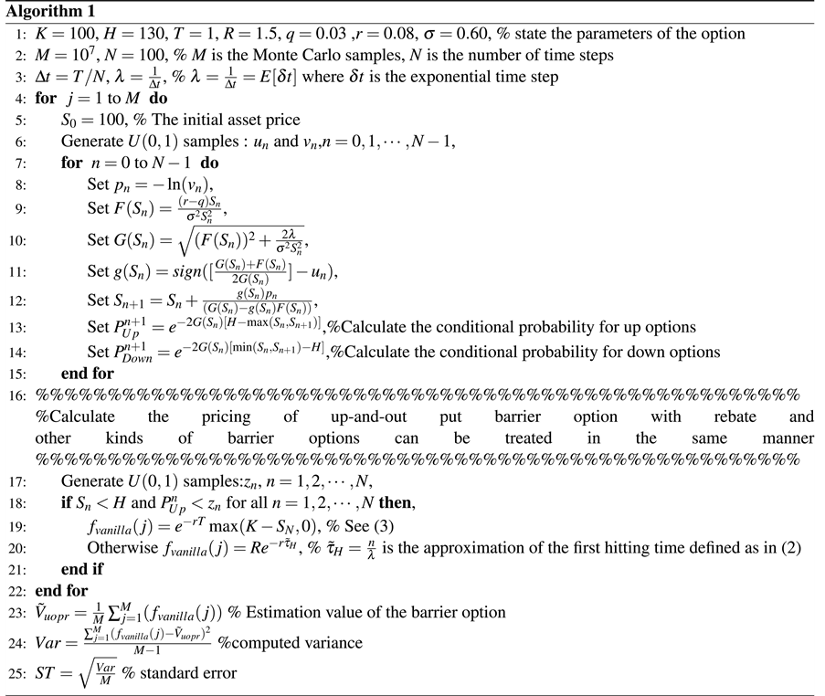
Appendix A
Algorithm of exponential timestepping with boundary test for the barrier options.