American Journal of Computational Mathematics
Vol.06 No.02(2016), Article ID:67205,14 pages
10.4236/ajcm.2016.62009
Group Method Analysis of MHD Mixed Convective Flow Past on a Moving Curved Surface with Suction
Dipika Rani Dhar1, Mohammad Abdul Alim2, Laek Sazzad Andallah3
1Department of Mathematics, Gouripur M.F.R. Government College, Comilla, Bangladesh
2Department of Mathematics, Bangladesh University of Engineering and Technology, Dhaka, Bangladesh
3Department of Mathematics, Jahangirnagar University, Dhaka, Bangladesh

Copyright © 2016 by authors and Scientific Research Publishing Inc.
This work is licensed under the Creative Commons Attribution International License (CC BY).
http://creativecommons.org/licenses/by/4.0/


Received 23 February 2016; accepted 6 June 2016; published 9 June 2016
ABSTRACT
The group-theorytic approach is applied for solving the problem of the unsteady MHD mixed convective flow past on a moving curved surface. The application of two-parameter groups reduces the number of independent variables by two, and consequently the system of governing partial differential equations with boundary conditions reduces to a system of ordinary differential equations with appropriate boundary conditions. The obtained ordinary differential equations are solved numerically using the shooting method. The effects of varying parameters governing the problem are studied. A comparison with previous work is presented.
Keywords:
Moving Curved Surface, MHD Flow, Two-Parameter Group-Theory Method, Buoyancy Parameter, Suction

1. Introduction
Applications of group-theory in fluid mechanics and boundary layer flow have received much attention by many researchers as the concepts of group theory are extensively used in similarity and non-similarity related problems. Group-theory method provides a powerful tool to nonlinear differential models. The transformation group theory approach is applied to present an analysis of the similarity problem of MHD mixed convective flow past on a moving curved surface with suction. The natural flow originates from body force variations in fluids, whereas the forced convection is generally introduced by moving a body through a quiescent fluid or by forcing a fluid past a stationary body. This flow regime is concerned with circumstances where in both the natural and forced mechanisms of the flow must be considered simultaneously. The laminar boundary layer flow due to such combined forced and natural convection i.e. mixed convection has received considerable attention for steady and unsteady situations in evaluating flow parameters for technical purposes. The problem of mixed convective boundary layer flow gained different dimensions in the manufacturing processes in industry. There has been great interest in the study of Magnetic Hydro-Dynamic (MHD) flow due to the effect of magnetic fields on the boundary layer flow control and on the performance of many systems using electrically conducting fields. This type of flow has attracted the interest of many researchers due to its applications in many engineering problems such as MHD generators, plasma studies, nuclear reactors, geothermal energy extraction etc.
Sparrow, Eichorn and Gregg [1] , were the first investigators, who dealt with the combined forced and free convective boundary layer flow about a vertical flat plate. The laws governing the motion of mixed convective boundary layer incompressible viscous fluid expressed in general orthogonal curvilinear co-ordinates are recently studied by Maleque [2] . Quiser Azam [3] studied mixed convection about the vertical developable flow surfaces with transpiration and heat flux effects. “Mixed convection boundary layer flow over a permeable vertical cylinder with prescribed surface heat flux” studied by Anuar Is hak et al. [4] . M.Y. Ali et al. [5] investigated similarity solutions for unsteady laminar boundary layer flow around a vertical heated curvilinear surface. Zakerullah [6] derived similarity solutions of some of possible cases of unsteady mixed convection by group theory without suction. Alam et al. [7] investigated “Magnetohydrodynamic free convection along a vertical wavy surface. S.M.M. EL-Kabeir et al. [8] studied Unsteady MHD combined convection over a moving vertical sheet in a fluid saturated porous medium with uniform surface heat flux. Dipika Rani Dhar [9] studied group- theory method on similarity solution of unsteady free convection flow from a moving vertical surface with suction and injection.
The mathematical technique used in the present analysis is two-parameter group transformation that leads to a similarity representation of the problem. Morgan [10] presented a theory that led to improvements over earlier similarity methods. Michal [11] extended Morgan’s theory. Group methods, as a class of methods which lead to a reduction of the number of independent variables, were first introduced by Birkoff [12] . He made use of one parameter group transformations to reduce a system of partial differential equations in two independent variables to a system of ordinary differential equations in one independent variable, the similarity variable. Morgan and Gaggioli [13] presented general systematic group formalism for similarity analysis, where a given system of partial differential equations was reduced to a system of ordinary differential equations.
In this work, the effect of MHD mixed convective flow past on a moving curved surface has been investigated. Problems are solved analytically using group methods and then numerically by Runge-Kutta shooting method. Under the application of two-parameter group, the governing partial differential equations are reduced to system of ordinary differential equations with the appropriate boundary conditions and then numerically using the sixth order Runge-Kutta shooting method known as Runge-Kutta-Butcher initial value solver of Butcher [14] together with the Nachtsheim-Swigert iteration scheme described by Nachtsheim and Swigert [15] . Programming codes have been written in FORTRAN 90 to implement shooting method for the present problem.
Attention has been taken on the evaluation of the velocity profiles as well as temperature profiles for selected values of parameters consisting ,magnetic parameter M, Prandtl number Pr, buoyancy parameter l1 and suction parameter Ew. The numerical results of the velocity profiles as well as temperature profiles are displayed graphically for different values of magnetic parameter M, Prandtl number Pr, buoyancy parameter l1 and suction parameter Ew. The post processing software TECPLOT has been used to display the numerical results. A comparison with previous work is presented.
2. Governing Equations
We consider the flow direction along the x-axis and η-axis and be defined in the surface over which the boundary layer is flowing. For simplicity  has been set such that ζ represents actual distance measured normal to the surface. The body force is taken as the gravitational force
 . The physical configuration is considered as shown in Figure 1.
The governing boundary layer equations of the flow field in general orthogonal curvilinear co-ordinates are:
Continuity equation

Figure 1. Physical model and co-ordinate system.
 (1)
(1)
Momentum equations
 (2)
(2)
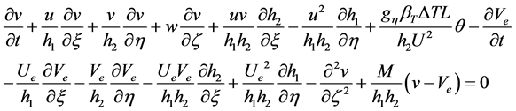 (3)
(3)
Energy equation
 (4)
(4)
With initial and boundary conditions
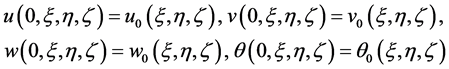 (5)
(5)

where

 is the magnetic parameter;
  is the magnetic induction;
  is the Prandtl number of the fluid;
  is
is
the thermal diffusivity.
From the continuity Equation (1), there exists two stream functions  and
and  such that

Applying h1 = 1 and h2 = ξ in Equations (2)-(4) we have
 (6)
(6)
 (7)
(7)
 (8)
(8)
With initial and boundary conditions
 (9)
(9)
3. Solution of the Problem
The problem is solved by applying a two parameter group transformation to the partial differential Equations (6)-(8). This transformation reduces the four independent variables  to one similarity variable
  and the governing Equations (6)-(8) are transformed to a system of ordinary differential equations in terms of the similarity variable γ.
3.1. The Group Systematic Formulation
Define the procedure is initiated with the group G, a class of transformation of two parameters  of the form
 (10)
(10)
S stands for t, x, h, z, Y, j, Ue, Ve, ∆T and q, CS and KS are real-valued and at least differentiable in their real arguments .
.
3.2. The Invariance Analysis
The transformation of the dependent variables and their partial derivatives are obtained from G via chain-rule operations
 (11)
(11)
where S stands for y, f, q. i.e.  etc.
etc.
Equation (6) is said to be invariantly transformed whenever
 (12)
(12)
Substitution from Equations (10) & (11) into Equation (12) yields


where 
In a similar manner, the invariant transform of (7) gives

where 
Similarly equation (8) is invariantly transformed giving

where 
The initial and boundary conditions being also invariant implies that kt = 0, kz = 0.
The invariant transformation of (6)-(8), the initial condition and the boundary conditions summarize in a group G of the form
 (13)
(13)
3.3. The Complete Set of Absolute Invariants
Our aim is to make use of group methods to represent the problem in the form of an ordinary differential equation (Similarity representation) in a single independent variable (Similarity variable). Then we have to proceed in our analysis to obtain a complete set of absolute invariants.
The complete set of absolute invariants is:
a)  is the absolute invariant of the independent variables t, x, h, z.
b)  are the five absolute invariants corresponding to the five dependent variables Y, j, Ue, Ve,q, ∆T.
A function  is an absolute invariant of a two-parameter group if it satisfies the following two first- order linear differential equations:
 (14a)
(14a)
 (14b)
(14b)
 etc.
etc.
 indicates the value of
  which yields the identity element of the group.
Independent Variables as Absolute Invariants
The absolute invariant  of the independent variables
  is determined using Equation (14)
 (15)
(15)
A successive elimination of  from Equations (15) yields
 (16a)
(16a)
 (16b)
(16b)
where 
Invoking the group given in Equation (13) and the definition of the α’s and β’s we get ,
,  thus
thus

From Equation (16b) we obtain , which means that γ is independent of η and γ is a function of t, ξ and
ζ; Solving Equations (16a) and (16b) implies 
Dependent Variables as Absolute Invariants
Similarly the absolute invariants of the dependent variables; Y, j, Ue, Ve, q are obtained from the group trans- formation (13),

A function  is absolute invariant of a two-parameter group if it satisfies the first-order linear differential equations
 (17)
(17)
The solution of Equation (17) gives
 (18)
(18)
In similar manner, we get
 (19)
(19)
 (20)
(20)
Since Ue(γ) and Ve(γ) are independent of ζ, whereas γ depends on ζ, it follows that Ue(γ) and Ve(γ) must be equal to constant, say one. Without loss of generality, the χ’s in Equations (18)-(19) are selected to the identity functions. So we can write
 (21)
(21)
 (22)
(22)
 (23)
(23)
Again ∆T is independent of ζ, whereas γ depends on ζ, it follows that G(γ) is equal to a constant, say G0. Without loss of generality G0 is equated to one. So
 (24)
(24)
4. The Reduction to the Ordinary Differential Equation
The system of ordinary differential Equations (6)-(8) eventually reduces to
 (25)
(25)
 (26)
(26)
 (27)
(27)
where
 (28)
(28)
and c’s are constant  and
and  are buoyancy parameter or mixed convection parameter.
Let in (28) c9/c10 = 1; then it follows that 
By considering c5 may be taken to be unity, we get from (28) the following

Now if we consider c8 = 1, (28) implies
 ,
, 
implies 
Evaluation of c’s implies .
.
Equations (25)-(27) gives u-momentum equation
 (29)
(29)
v-momentum equation
 (30)
(30)
Energy equation
 (31)
(31)
with related boundary conditions:
 (32)
(32)
Equations (29)-(31) together with the boundary condition (32) are solved numerically using the sixth order Runge-Kutta shooting method known as Runge-Kutta-Butcher initial value solver of Butcher (1974) together with the Nachtsheim-Swigert iteration scheme described by Nachtsheim and Swigert (1965).
The numerical results of the velocity profiles as well as temperature profiles for different values of magnetic parameter M, Prandtl number Pr, buoyancy parameter l1 and suction parameter Ew will be discussed and display graphically.
5. Results and Discussion
The main objective of the present study is to analyze the effect of MHD mixed-convection flow on a moving curved surface. Figure 2 and Figure 3 illustrate the dimensionless velocity profiles along ξ and η directions, respectively for fixed values of Pr = 0.73, λ1 = −13.29, λ2 = −0.76 and Ew = 1.53 with several values of M. Since magnetic parameter is inversely proportional with Reynold number, Re so increasing values of the magnetic parameter M decreases the flow rate in the velocity boundary layer thickness. It has been seen from Figure 2, due to moving surface the u-velocity profiles at the boundary surface fall down slowly then u-velocity profiles decreases rapidly corresponds to opposing flow up to the peak points g = 3.25, 2.85, 2.55 and then velocity inte-

Figure 2. Dimensionless u-velocity profiles against similarity variable γ for different values of M (Pr,λ1,λ2 and Ew are fixed).

Figure 3. Dimensionless v-velocity profiles against similarity variable γ for different values of M (Pr,λ1,λ2 and Ew are fixed).
grate slowly for magnetic parameter M = 0.9, 0.09, 0.01. It is observed from Figure 3 that v-velocity profiles decreases with the increasing values of magnetic parameter M that is velocity profiles meet together at the position of g = 3.4 and cross the sides. It has been seen from Figure 4 when the Prandtl number Pr = 0.80, 0.74, 0.73, 0.70 u-velocity profiles fall down up to the position of g = 2.05, 2.15, 2.50 and from that positions of g, u-velocity profiles rising up and finally approach to one. In Figure 5 shown that the maximum values of v-velocities are recorded as 1.9452, 1.9515, 1.9580 and 1.9768 for Prandtl number Pr = 0.75, 0.74, 0.73, 0.70 at the position of g = 1.30, 1.35, 1.35, 1.40 respectively. It is observed from Figure 6 that u-velocity profiles de-

Figure 4. Dimensionless u-velocity profiles against similarity variable γ for different values of Pr (M, λ1, λ2 and Ew are fixed).

Figure 5. Dimensionless v-velocity profiles against similarity variable γ for different values of Pr (M, λ1, λ2 and Ew are fixed).

Figure 6. Dimensionless u-velocity profiles against similarity variable γ for different values of Ew (M, λ1, λ2 and Pr are fixed).
creases with the increasing values of suction parameter Ew. It has been seen from Figure 7 that as the suction parameter Ew increases, the v-velocity profiles increases up to the position of g = 1.50, 1.50, 1.35, 1.30 and from that positions of g velocity profiles decreases with the increasing values of suction parameter Ew. From Figure 8, it is observed that owing to the effect of the buoyancy parameter λ1 = −13.29, −12.80, −12, −11, u-velocity profiles decreases up to the position of g = 2.10, 1.85, 1.65, 1.45 and from those positions of g, u-velocities integrate rapidly and increases for increasing values of g. In Figure 9 it is shown that the v-velocities of the fluid against g decreases for increasing values of buoyancy parameter λ1. The maximum values of the v-velocity are found to be

Figure 7. Dimensionless v-velocity profiles against similarity variable γ for different values of Ew (M, λ1, λ2 and Pr are fixed).

Figure 8. Dimensionless u-velocity profiles against similarity variable γ for different values of λ1 (M, Ew, λ2 and Pr are fixed).

Figure 9. Dimensionless v-velocity profiles against similarity variable γ for different values of λ1 (M, Ew, λ2 and Pr are fixed).
1.9628, 1.9548, 1.9453 and 1.9334 for λ1 = −13.29, −12.80, −12, −11 respectively. It is noted that the v-velocity decreases by approximately1.5% as λ1 increases from −13.29 to −11. Figure 10 illustrates for fixed values of Pr = 00.73, λ1 = −13.29, λ2 = −0.76 and Ew = 1.53 the temperature profiles decreases with the increasing values of magnetic parameter M. Figure 11 and Figure 12 display the results for the temperature profiles. It is observed from the Figure 11 and Figure 12 that the thermal boundary layer thickness decrease for the increasing values of Prandtl number Pr and suction parameter respectively. Figure 13 shows the small increment on the temperature for increasing values of the buoyancy parameter λ1.

Figure 10. Dimensionless temperature profiles against similarity variable γ for different values of Pr (M, λ1, λ2 and Ew are fixed).

Figure 11. Dimensionless temperature profiles against similarity variable γ for different values of Pr (M, λ1, λ2 and Ew are fixed).

Figure 12. Dimensionless temperature profiles against similarity variable γ for different values of Ew (M, λ1, λ2 and Pr are fixed).

Figure 13. Dimensionless temperature profiles against similarity variable γ for different values of λ1 (M, Ew, λ2 and Pr are fixed).

Table 1. Comparison of the values of ,
,  and
and  with Maleque Kh.A. [2] and Present work for the variation of Prandtl number Pr while M = 0.0, Ew = 0 and
 .
.
6. Comparison with Previous Work and Code Validation
A comparison of the present numerical results of ,
,  and
and  with this, obtained by Maleque Kh.A. [2] , is depicted in Table 1. Here, the parameters M and Ew are igno red with different values of Prandtl number Pr. It is evidently seen from Table 1 that the current results are concurrence with the solution of Maleque Kh.A. [2] .
Cite this paper
Dipika Rani Dhar,Mohammad Abdul Alim,Laek Sazzad Andallah, (2016) Group Method Analysis of MHD Mixed Convective Flow Past on a Moving Curved Surface with Suction. American Journal of Computational Mathematics,06,74-87. doi: 10.4236/ajcm.2016.62009
References
- 1. Sparrow, M.E., Eichorn, R. and Gregg, L.J. (1959) Combined Forced and Free Convection in a Boundary Layer Flow.
- 2. Maleque, Kh.A. (1995) Similarity Solutions of Combined Forced and Free Convection Laminar Boundary Layer Flows in Curvilinear Coordinates. M. Phil. Thesis, Department of Mathematics, BUET, Dhaka.
- 3. Azam, Q. (1998) Mixed Convection about the Vertical Developable Flow Surfaces with Transpiration and Heat Flux Effects. M. Phil. Thesis, Department of Mathematics, BUET, Dhaka.
- 4. Ishak, A. and Bachok, N. (2009) Mixed Convection Boundary Layer Flow over a Permeable Vertical Cylinder with Prescribed Surface Heat Flux. European Journal of Scientific Research, 34, 46-54.
- 5. Ali, M.Y. and Hafez, M.G. (2012) A Case of Similarity Solutions for Unsteady Laminar Boundary Layer Flow in Curvilinear Surface. ARPN, 7, No.6.
- 6. Zakerullah, Md. (2001) Similarity Analysis. Thesis, Bangladesh University of Engineering and Technology, Dhaka.
- 7. Alam, K.C.A., Hossain, M.A. and Rees, D.A.S. (1997) Magnetohydrodynamic Free Convection along a Vertical Wavy Surface. International Journal of Applied Mechanics and Engineering, 1, 555-566.
- 8. EI-kabir, S.M.M., Rashad, A.M., Subba, R. and Gorla, R. (2007) Unsteady MHD Combined Convection over a Moving Vertical Sheet in a Fluid Saturated Porous Medium with Uniform Surface Heat Flux. Science Direct Mathematical and Computer Modelling, 46, 384-397.
- 9. Dhar, D.R. (2007) Group-Theory Method on Similarity Solution of Unsteady Free Convection Flow from a Moving Vertical Surface with Suction and Injection. M. Phil. Thesis, Department of Mathematics, BUET, Dhaka.
- 10. Moran, A.G.A. (1962) The Reduction by One of the Number of Independent Variables in Some Systems of Partial Differential Equations. Quarterly Journal of Mathematics, 3, 250-259.
http://dx.doi.org/10.1093/qmath/3.1.250 - 11. Michal, A.D. (1952) Differential Invariants and Invariant Partial Differential Equations under Continuous Transformation Groups in Normal Linear Spaces. Proceedings of the National Academy of Sciences of the United States of America, 37, 623-627.
http://dx.doi.org/10.1073/pnas.37.9.623 - 12. Birkoff, G. (1948) Mathematics for Engineers. Electrical Engineering, 67, 1185.
- 13. Moran, M.J. and Gaggioli, R.A. (1968) A New Systematic Formalism for Similarity Analysis, with Application to Boundary Layer Fows. Technical Summary Report No. 918, U.S. Army Mathematics Research Center.
- 14. Butcher, J.C. (1974) Implicit Runge-Kutta Process. Mathematics of Computation, 18, 50-55.
http://dx.doi.org/10.1090/S0025-5718-1964-0159424-9 - 15. Nachtsheim, P.R. and Swigert, P. (1965) Satisfaction of Asymptotic Boundary Conditions in Numerical Solutions of Systems of Non-Linear Equations of Boundary-Layer Type. NASA TN-D3004.