American Journal of Computational Mathematics
Vol.3 No.1A(2013), Article ID:30854,7 pages DOI:10.4236/ajcm.2013.31A003
On Constructing Approximate Convex Hull
Computer Vision and Cybernetics Research Group, School of Engineering and Computer Science, Independent University, Dhaka, Bangladesh
Email: mzhossain@gmx.com, aminmdashraful@ieee.org
Copyright © 2013 M. Zahid Hossain, M. Ashraful Amin. This is an open access article distributed under the Creative Commons Attribution License, which permits unrestricted use, distribution, and reproduction in any medium, provided the original work is properly cited.
Received January 29, 2013; revised February 28, 2013; accepted March 13, 2013
Keywords: Convex Hull; Approximation Algorithm; Computational Geometry; Linear Time
ABSTRACT
The algorithms of convex hull have been extensively studied in literature, principally because of their wide range of applications in different areas. This article presents an efficient algorithm to construct approximate convex hull from a set of n points in the plane in  time, where k is the approximation error control parameter. The proposed algorithm is suitable for applications preferred to reduce the computation time in exchange of accuracy level such as animation and interaction in computer graphics where rapid and real-time graphics rendering is indispensable.
1. Introduction
The construction of planar convex hull is one of the most fundamental problems in computational geometry. The applications of convex hull spread over large number of fields including pattern recognition, regression, collision detection, area estimation, spectrometry, topology, etc. For instance, computer animation, the most crucial section of computer gaming, requires fast approximation for real-time response. Consequently, it is evidential from literature that numerous studies focus on fast approximation of different geometric structures in computer graphics [1,2]. Moreover, the construction of exact and approximate convex hull is used as a preprocessing or intermediate step to solve many problems in computer graphics [3,4].
Convex hull for a given finite set  of
of  points where
  denotes the
  -dimensional Euclidean space, is defined as the smallest convex set that contains all the
  points. A set
  is convex if for two arbitrary points
 , the line segment
  is entirely contained in the set
 . Alternatively, the convex hull can be defined as the intersection of all halfspaces (or half-planes in
 ) containing
 . The main focus of this article is limited on the convex hull in Euclidean plane
 .
.
2. Previous Work
Because of the importance of convex hull, it is natural to study for improvement of running time and storage requirements of the convex hull algorithms in different Euclidean spaces. Graham [5] published one of the fundamental algorithms of convex hull, widely known as Graham’s scan as early as 1972. This is one of the earliest convex hull algorithms with  worst-case running time. Graham’s algorithm is asymptotically optimal since
  is the lower bound of planar convex hull problem. It can be shown [6] that
  is a lower bound of a similar but weaker problem of determining the points belonging to the convex hull, not necessarily producing them in cyclic order.
However, all of these lower bound arguments assume that the number of hull vertices  is at least a fraction of
 . Another algorithm due to Jarvis [7] surpasses the Graham’s scan algorithm if the number of hull vertices
  is substantially smaller than
 . This algorithm with
  running time is known as Jarvis’s march. There is a strong relation between sorting algorithm and convex hull algorithm in the plane. Several divide-and-conquer algorithms including MergeHull and QuickHull algorithms of convex hull modeled after the sorting algorithms [8] and the first algorithm Graham’s [5] scan uses explicit sorting of points.
In 1986, Kirkpatrick and Seidel [9] proposed an algorithm that computes the convex hull of a set of  points in the plane in
  time. Their algorithm is both output sensitive and worst case optimal. Later, a simplification of this algorithm [9] was obtained by Chan [10]. In the following year Melkman [11] presented a simple and elegant algorithm to construct the convex hull for simple polyline. This is one of the on-line algorithms which construct the convex hull in linear time.
Approximation algorithms for convex hull are useful for applications including area estimation of complex shapes that require rapid solutions, even at the expense of accuracy of constructed convex hull. Based on approximation output, these algorithms of convex hull could be divided into three groups—near, inner, and outer approximation algorithms. Near, inner, and outer approximation algorithms compute near, inner, and outer approximation of the exact convex hull for some point set respectively.
In 1982, Bentley et al. [12] published an approximation algorithm for convex hull construction with  running time. Another algorithm due to Soisalon-Soininen [13] which uses a modified approximation scheme of [12] and has the same running time and error bound. Both of the algorithms are the inner approximation of convex hull algorithm. The proposed algorithm in this article is a near approximation algorithm of
  running time.
3. Approximation Algorithm
Let  be the finite set of
  points in general position and the (accurate) convex hull of
  be
be . Kavan, Kolingerova, and Zara [14] proposed an algorithm with
  running time which partitions the plane
  into
into  sectors centered in the origin. Their algorithm requires the origin to be inside the convex hull. (It is possible to choose a point
  and translate all the other points of
  accordingly using additional steps in their algorithm). Conversely, we partition the plane
  into
into  vertical sector pair with equal central angle
  in the origin and for our algorithm the origin
  could be located outside of the convex hull. The sets represent the vertically opposite sectors that form the vertical sector pairs defined as
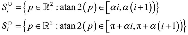
where,  and the central angle
 . Then, the sets
  and
and  denote the points belonging to the set
  in sectors
  and
and  respectively. Formally,

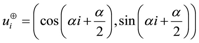
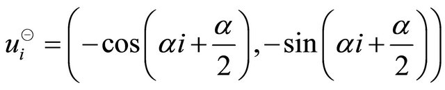
A pair of unit vectors  and
and  obtain in
  th vertical sector pair as
The maximum projection magnitudes in the directions of  and
and  are (Figure 1)
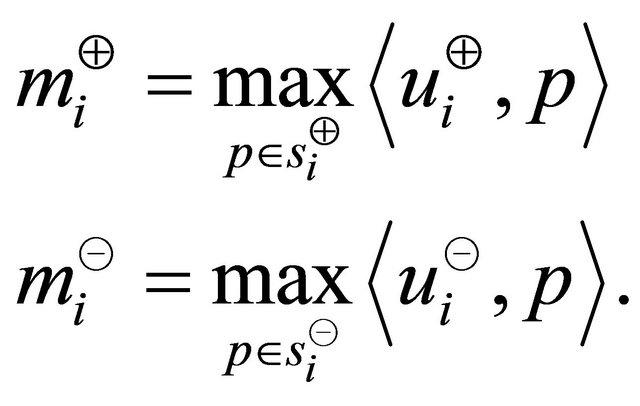
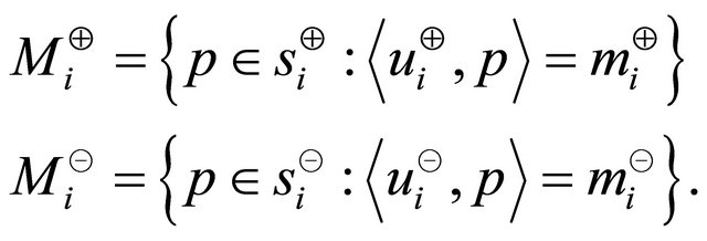
The definition of max function is extend to return  for no parameter. The sets of points which provide the maximum projection magnitude in the sectors of
  th vertical sector pair are
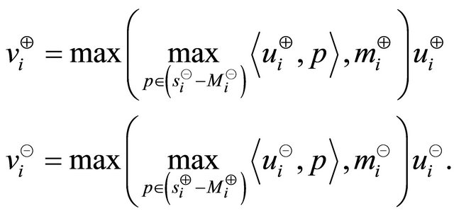
The vectors that produce the maximum magnitude in the directions of  and
and  for some points in the
  th vertical sector pair are
The magnitude of the vectors  and
and  could be
  for the
  th vertical sector pair containing less than two points. The sets
  and
and  containing all the finite vectors in the ranges
  and
and , are
, are
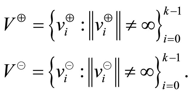
Let,  and
and  contains at least three terminal points of the vectors in general position to construct the convex hull.

Figure 1. An example of convex hull CH16 constructed using proposed algorithm based on a set of 50 points.
The convex hull approximation of  vertical sector pairs according to the proposed algorithm in this article is:
4. Implementation
The input of the algorithm  is a set of
  points in general position. For simplicity, we assume that the origin
  and
and . (This assumption can be achieved by taking a point arbitrarily close to the origin instead of the origin itself, within the upper bound of error calculated in Section 5) (Figure 2).
We also assume that at least two vertical sector pairs together contains minimum three points (where none of these two are empty). The assumption can be reduced to one of the requirements of minimum three points input (i.e., ) of convex hull. To illustrate that, let us consider
  and
and  to be two points in
  such that
  where
where  is the origin. Such two points do exist if no three points are collinear in
  (i.e., the points of
  are in general position). If
  is the bisector of
 , then adding the angle of
  from positive
  -axis as an offset to every vertical sector pair ensures that all the input points cannot be in the same vertical sector pair. Thus, the assumption is satisfied. Alternatively, if less than three absolute values in
  are finite, then for each
 , assign
  to
to  and
and  where these are infinite. (The next pa-
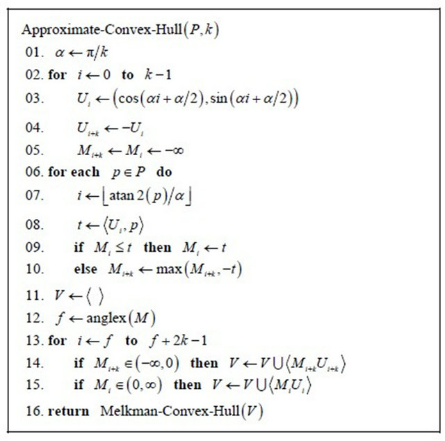
Figure 2. The proposed algorithm to compute an approximate convex hull in  time from inputs P and
  where
where  is a set of
  points in the plane and k is the number of vertical sector pair partitioning the plane.
ragraph contains details about M.) Therefore, the number of points in  must be at least three.
A circular array  is used to contain the
  pairs of unit vectors of all the
  vertical sector pairs and another circular array
  is used to hold the number of
  pairs of maximum projection magnitude in all the
  vertical sector pairs. Both circular arrays have the same size of
  and use zero based indexing scheme. The function atan2 is a variation of function arctan with point as a parameter. The function returns the angle in radians between the point and the positive
  -axis of the plane in the range of
 . The function anglex searches sequentially for the index of maximum angular distance between two consecutive positive finite vectors (computed using projection magnitude with index referring angle). If the index is
  such that maximum angle occurs in between
  and
and , the anglex function returns
 . The final convex hull is constructed using Melkman’s [11] algorithm from set of
  points which are the terminal points of finite vectors computed in steps 14 and 15. If the first three points of
  are collinear, displacing one of these points within the error bound solves the problem.
Since the vertices of the convex hull produced by the proposed algorithm are not necessarily in the input point set , the algorithm cannot be applied straight away to solve some other problems. Let us consider another circular array
  of
of  size which used to contain the points generating the inner products of
 . Adding the point
  instead of
  to the sequence
  in Steps 14 and 15 ensures that the vertices of the convex hull will be the points from
 . These modifications of the algorithm allow us to solve some problems including approximate farthest-pair problem but increase the upper bound of error (described in Section 5) to
 .
.
5. Error Analysis
There are different schemes for measuring the error of an approximation of the convex hull. We measured the error as distance from point set of accurate convex hull . The distance of an arbitrary point
  from a set
  is defined as
Formally the approximation error  can be defined as
It is sufficient to determine the upper bound of error  of the approximate convex hull
 . Let,
  be be a point lying outside of the convex hull
  and
and  be the origin. Suppose that,
  is an edge of the approximate convex hull (as shown in Figure 3).
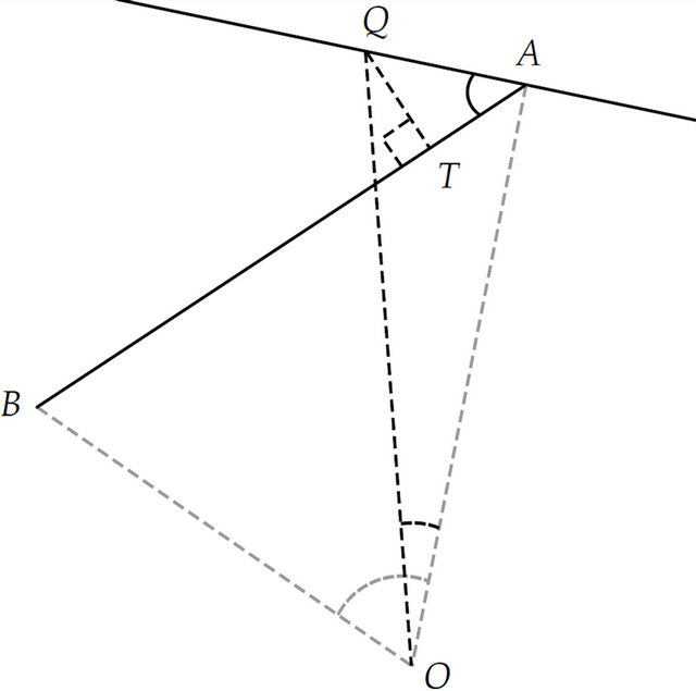
Figure 3. The approximation error of the proposed algorithm measured as a distance  of the point
  lying outside of the approximate convex hull with an edge
 .
.
Therefore, the distance of the point  from the
 is
is
 .
.
The distance of the point  from vertex
  is
is . Thus,
 .
.
Let,  and
and . Thus we obtain
It follows that the minimum distance  directly depends on
  which is denoted as function
 . Thus, the upper bound of approximation error
  is
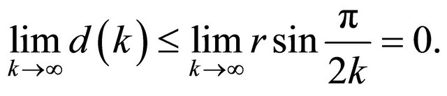
is . If
. If  approaches to infinity, the
  converges to
 .
.
For instance, when k approaches to a large value, the area approximation error of the circle is reducing exponentially as shown in Figure 4. Therefore, this algorithm is more optimize than the KKZ algorithm [14] with respect to error bound as shown in Figure 5.
6. Correctness
Theorem 1. The approximation algorithm produces the convex hull from a set of points in  correctly within the prescribed error bound.
Proof. Since, Melkman’s algorithm can construct the convex hull correctly for points on a simple polygonal chain, it suffices to prove that the sequence of points  denotes a simple polygonal chain. (Melkman [11] published the on-line algorithm of convex hull with formal proof of correctness in 1987).
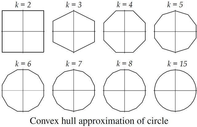
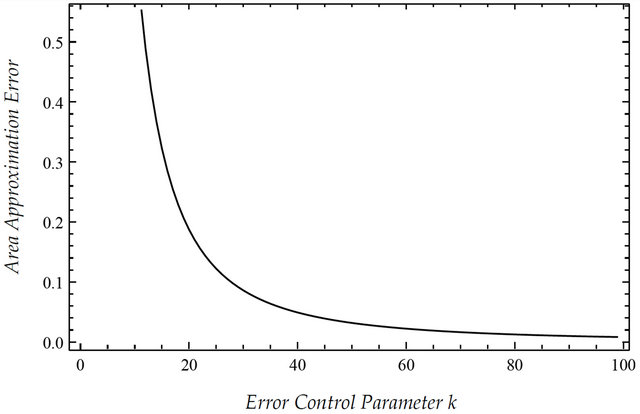
Figure 4. The graph showing approximation error of a circle area with respect to error control parameter  where the number of input points is
  lying on a circle of radius 4 units.

Figure 5. The graph representing the relation between the error control parameter  and upper bound of error
 . The upper error bounds
  and
and  are calculated in this article and in [14] (i.e., KKZ Algorithm) respectively where
  is unit in the graph.
Suppose that, the plane  is partitioned into
  vertical sector pairs which correspond to the sequence
 of
of  simple sectors. The sequence
 of sectors is ordered according to the angle measured anticlockwise. If
  is a half-line (denoting the set of points on the half-line) from the origin in the direction of the unit vector of the sector
 , then the sequence
 represents all the half-lines correlated with the sequence
 . According to the algorithm all the points of
  must be distinct (as referred in steps 9-10) and lying on some of the half-lines of
 . The sequence of half-lines
  where each contained at least one point from
 , is
, is
Each half-line  can contain at most two points of
 . Let,
  are points on each halfline
  such that
 . If a half-line
contains only one point of , the length of virtual
  is zero with
  and
and  refer to the same point of
  (e.g.,
  contains only one point in the Figure 6). Let
  denotes the angle from
  to
to  where
where  and
and  are half-lines from the origin. Since the angle between two consecutive half-lines
  and
and  (because
  for our assumptions
  and
and  in the algorithm), no two line segments
  and
and  intersect each other, for all
 . However, the line segment
  could cross the polygonal chain
  if the angle
 . The equation of
  (derived using the law of sines and basic properties of triangle) also illustrates this fact mathematically for
  (as shown in the Figure 6).

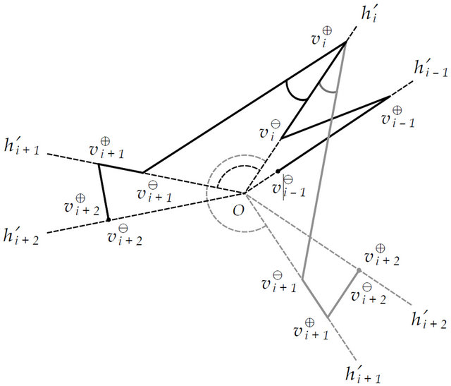
Figure 6. The proof of correctness of the algorithm that consider both the simple and non-simple variation of polygonal chain  with
with  and
and .
.
The solution with minimum magnitude of the above equation is negative for , even if
 . Thus the line segment
  could intersect with the edges of the polygonal chain only if
 . If the maximum angle between two consecutive half-lines is
  for some
 , then anglex function returns the index
  that ensures the construction a simple polygonal chain
  where
where  and all the indices are modulo
 . Thus the sequence of points
  represents a simple polygonal chain. (It is possible to prove the algorithm obtained by interchanging the steps 14 and 15, using a similar method).
Theorem 2. If  is the number of input points and
  is the number of vertical sector pairs in
 , then the running time of the proposed algorithm is
 .
.
Proof. Let us estimate the running time for each part of the algorithm to prove that the algorithm compute the approximate convex hull in  time. It is clear that, the initialization steps 2-5 take
  time. Since, the next loop of steps 6-10 iterates for each point
 , thus it takes
  time considering constant time for floor function. According to the description of anglex function in Section 4, the function can be implemented in
  time because it requires
  iterations to compute the index. The loop of steps 13-15 takes
  time and Melkman’s [11] algorithm runs in linear time. Steps 1 and 11 require constant time. Thus the running time of the algorithm is
 .
.
7. Conclusion
Geometric algorithms are frequently formulated under the non-degeneracy assumption or general position assumption [15] and the proposed algorithm in this article is also not an exception. To make the implementation of the algorithm robust an integrated treatment for the special cases can be applied. There are other general techniques called perturbation schemes [16,17] to transform the input into general position and allow the algorithm to solve the problem on perturbed input. Both symbolic perturbation and numerical (approximation) perturbation (where perturbation error is consistent with the error bound of the algorithm) can be used on the points of  to eliminate degenerate cases.
8. Acknowledgements
This research is supported by a grant from Independent University Bangladesh (IUB).
REFERENCES
- J. Hu and H. Yan, “Polygonal Approximation of Digital Curves Based on the Principles of Perceptual Organization,” Pattern Recognition, Vol. 30, No. 5, 2006, pp. 701- 718. doi:10.1016/S0031-3203(96)00105-7
- R. Bellman, B. Kashef and R. Vasudevan, “Mean Square Spline Approximation,” Journal of Mathematical Analysis and Applications, Vol. 45, No. 1, 1974, pp. 47-53. doi:10.1016/0022-247X(74)90119-X
- J. T. Klosowski, M. Held, J. S. B. Mitchell, H. Sowizral, and K. Zikan, “Efficient Collision Detection Using Bounding Volume Hierarchies of k-DOPs,” IEEE Transactions on Visualization and Computer Graphics, Vol. 4, No. 1, 1998, pp. 21-36. doi:10.1109/2945.675649
- X. Zhang, Z. Tang, J. Yu and M. Guo, “A Fast Convex Hull Algorithm for Binary Image,” Informatica (Slovenia), Vol. 34, No. 3, 2010, pp. 369-376.
- R. L. Graham, “An Efficient Algorithm for Determining the Convex Hull of a Finite Planar Set,” Information Processing Letters, Vol. 1, No. 4, 1972, pp. 132-133. doi:10.1016/0020-0190(72)90045-2
- A. C.-C. Yao, “A Lower Bound to Finding Convex Hulls,” Journal of the ACM, Vol. 28, No. 4, 1981, pp. 780-787. doi:10.1145/322276.322289
- R. A. Jarvis, “On the Identification of the Convex Hull of a Finite Set of Points in the Plane,” Information Processing Letters, Vol. 2, No. 1, 1973, pp. 18-21. doi:10.1016/0020-0190(73)90020-3
- F. P. Preparata and M. I. Shamos, “Computational Geometry: An Introduction,” Springer-Verlag Inc., New York, 1985.
- D. G. Kirkpatrick and R. Seidel, “The Ultimate Planar Convex Hull Algorithm,” SIAM Journal on Computing, Vol. 15, No. 1, 1986, pp. 287-299. doi:10.1137/0215021
- T. M. Chan, “Optimal Output-Sensitive Convex Hull Algorithms in Two and Three Dimensions,” Discrete & Computational Geometry, Vol. 16, No. 4, 1996, pp. 361- 368. doi:10.1007/BF02712873
- A. A. Melkman, “On-Line Construction of the Convex Hull of a Simple Polyline,” Information Processing Letters, Vol. 25, No. 1, 1987, pp. 11-12. doi:10.1016/0020-0190(87)90086-X
- J. L. Bentley, F. P. Preparata and M. G. Faust, “Approximation Algorithms for Convex Hulls,” Communications of the ACM, Vol. 25, No. 1, 1982, pp. 64-68. doi:10.1145/358315.358392
- E. Soisalon-Soininen, “On Computing Approximate Convex Hulls,” Information Processing Letters, Vol. 16, No. 3, 1983, pp. 121-126. doi:10.1016/0020-0190(83)90062-5
- L. Kavan, I. Kolingerova and J. Zara, “Fast Approximation of Convex Hull,” Proceedings of the 2nd IASTED International Conference on Advances in Computer Science and Technology, ACTA Press, Anaheim, 2006, pp. 101-104.
- J. O’Rourke, “Computational Geometry in C,” 2nd Edition, Cambridge University Press, New York, 1998. doi:10.1017/CBO9780511804120
- H. Edelsbrunner and E. P. Mücke, “Simulation of Simplicity: A Technique to Cope with Degenerate Cases in Geometric Algorithms,” ACM Transactions on Graphics, Vol. 9, No. 1, 1990, pp. 66-104. doi:10.1145/77635.77639
- I. Z. Emiris, J. F. Canny and R. Seidel, “Efficient Perturbations for Handling Geometric Degeneracies,” Algorithmica, Vol. 19, No. 1-2, 1997, pp. 219-242. doi:10.1007/PL00014417
Appendix
The article describes a near approximation algorithm for convex hull however it is possible to extend the concept for inner as well as outer approximation algorithms for convex hull. An illustration of inner approximate convex hull algorithm is shown in Figure 7.
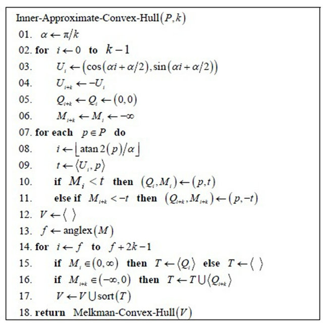
Figure 7. The proposed algorithm to compute an inner approximate convex hull in  time from inputs
  and
and  where
where  is a set of
  points in the plane and
  is the number of vertical sector pair partitioning the plane.