American Journal of Computational Mathematics
Vol.3 No.1(2013), Article ID:29076,11 pages DOI:10.4236/ajcm.2013.31003
A Derivative-Free Optimization Algorithm Using Sparse Grid Integration
Department of Mathematics and Statistics, York University, Toronto, Canada
Email: chensy@mathstat.yorku.ca, stevenw@mathstat.yorku.ca
Received October 2, 2012; revised November 12, 2012; accepted December 1, 2012
Keywords: Nonlinear Programming; Derivative Free Optimization; Sparse Grid Numerical Integration; Conditional Moment
ABSTRACT
We present a new derivative-free optimization algorithm based on the sparse grid numerical integration. The algorithm applies to a smooth nonlinear objective function where calculating its gradient is impossible and evaluating its value is also very expensive. The new algorithm has: 1) a unique starting point strategy; 2) an effective global search heuristic; and 3) consistent local convergence. These are achieved through a uniform use of sparse grid numerical integration. Numerical experiment result indicates that the algorithm is accurate and efficient, and benchmarks favourably against several state-of-art derivative free algorithms.
1. Introduction
Derivative-based methods can be very efficient and have been widely used in solving optimization problems. In many applications, however, the derivative of an objecttive function might be unavailable, unreliable, or very costly to compute. Many scientific and engineering optimization problems fall into this category [1]. For example, in the helicopter rotor blade design problem [2], the objective function can only be evaluated by very expensive simulation. Similar problems include the nonlinear optimization parameter tuning problem [3], medical image registration [4], dynamic pricing [5], and community groundwater problem [6]. Therefore, derivative-free methods must be used in these situations. For these problems, not only the derivative information is not available, the function evaluation could be inaccurate or noisy most of times as well. Hence, an algorithm needs the capability to generate robust searching directions without using derivative and without overly relying on individual function evaluations.
There are several commonly used derivative-free algorithms in the literature. The classical Nelder-Mead method [7] is based on simplicies and various operations defined on these simplicies. The method evaluates the objective function on a finite number of points, and decides which operation to perform accordingly. The method is simple and able to follow the curvature of the objective function. Pattern search or directional direct search algorithm [8,9] defines a set of directions beforehand, such as positive spanning sets, positive bases or just the coordinates in its simplest form, and tests one candidate point on each of these directions in a so called polling step. An optional search step could proceed the polling step to accelerate the algorithm opportunistically, in which the algorithm makes use of some known properties, heuristics, or a surrogate model on a finite number of points. The implicit-filtering method [10] is a line search method based on the simplex gradient, which is computed based on the function values at the vertices of a simplex set. DFO method [11], Powell’s method [12] and Wedge method [13] are essentially trust-region methods; however, additional steps are executed since in the derivative free optimization a quadratic or linear interpolating or regression model does not necessarily improve when the trust-region radius is reduced. For extreme problems where the mathematical structure is complex or poorly understood, other heuristic optimization algorithms such as genetic algorithms, simulated annealing, artificial neural networks, tabu-search and particle swamp are also used as methods of a last resort. An excellent discussion of several commonly used derivative-free optimization methods can be found in [14].
We point out that all these derivative-free algorithms are local optimizer, i.e., only convergence to a local optimal point is guaranteed. However, on the other hand, all these algorithms are highly capable of filtering out noises, escape from inferior local optimums, and often return a fairly satisfactory solution. These widely used and successful designs clearly convey a common principle: for cases like the helicopter rotor blade design problem [2], where each function evaluation is an expensive simulation and is known to be noisy, generating robust and efficient searching directions has the highest priority. It does not mean that one can not conduct derivative-free global optimization. As a matter of fact, many derivative-free global optimization algorithms have been developed with different targeted application areas, for example, the particle swarm method, Mesh adaptive direct search (MADS) [15], DIviding RETangles (DIRECT) [16], and Multileve coordinate search (MCS) [17]. More interestingly, some of the above local derivative-free algorithms have been extended to solve global optimization problems, for example, the global Direct Search, see Section 13.3 [14] and references therein. It appears that four categories of algorithms, with or without derivative, seeking local or global optimums, all find their suitable application areas.
In this paper, our goal is to generate high-quality local optimal solutions efficiently. Hence in this paper, we are concerned with the following optimization problem:
 (1)
(1)
where , but is expensive to evaluate. In many applications, such as the helicopter rotor blade design problem [2],
  is known to be smooth, but has no analytical form, and one can only rely on expensive simulations or experiments to evaluate function values. The measurements could be inaccurate or noisy though the function
  itself is known to be smooth, see [14]. Furthermore, derivatives or reliable approximation are not available.
  could have many local optimums as well. The decision variable x is subject to a box constraint
 . For example, in the parameter tubing problem [3], B is a theoretically or empirically reasonable range of the parameters to be tuned.
Our research is motivated by Wang et al. [18], where the authors proposed a novel derivative free global optimization method. In this iterative method, the integral of the objective function over a local neighbourhood of each iterate is computed, which further determines the next iterate. The authors showed that if the neighbourhood size could be chosen properly at each iterate, the algorithm converges to a global optimum. The authors demonstrated a few examples, where the algorithm successfully found global optimums while several other commonly used derivative-free methods and even derivative-based methods failed.
We have a different view of the integration based derivative free optimization method. First of all, we use the integration to define the searching directions, rather than the iterates as did in [18]. We found that it is more efficient to use the integration to define the search direction. The integration based searching direction uses information from multiple function evaluations at strategically located points, which avoids unduly relying on the gradient information at the current iterate. This is especially important since the function evaluations are noisy, especially when obtained from simulation or physical measurements, hence the local gradient, even if available or can be approximated, has poor quality. Secondly, our focus is on generating high quality local optimum efficiently, rather than seeking a global optimum. This moderate goal actually enable us to search more effectively. Finding global optimum and proving its global optimality is known to be hard. Though [18] shows the existence of a series of neighbourhood sizes such that their algorithm can find a global optimum, the exact neighbourhood size is not given in theory, nor specified algorithmically. In this paper, we design a two stage searching strategy, which aims at achieving a good balance of global coverage and local optimality.
First, we divide the solution seeking process into two stages: the global probing stage and the local convergence stage. In the global probing stage, the algorithm search for high region of the feasible domain for a maximization problem; while in the local convergence stage, the algorithm converges to peaks of the high region found in the first stage. The first stage steps are typically large; and the second stage steps are small. We update the neighbourhood size differently in the two stages, which suites the different purposes of the two stages well.
Accordingly, we prove that in the local convergence stage the algorithm always generates locally improving directions and converges; while in the global probing stage, we are able to show that the algorithm can generate searching directions towards a global optimum but against a local attraction for the mixture model functions commonly appeared in statistics optimization.
We not only develop new theories to support our new perspective, but also design critical algorithmic components accordingly. Our new line search method is a greedy algorithm which appears to have good numerical performance. In the contrast, [18] does not use line search at all. Our strategy to select the starting point is also new. It is well-known that the starting point is important for nonlinear optimization problem. However, most nonlinear optimization algorithms, including [18], rely on user defined starting points or starting from zero mechanically. We provides an innovative approach here: we start from the center of gravity of the whole feasible region, which is again computed from integration with function values as weights. Hence the starting point is close to the global optimum.
Secondly, we use the modern sparse grid numerical integration method (Smolyak 1960) in computing the local integration. The sparse grid method is highly efficient for functions with moderate dimensions, and has been widely used in engineering, finance, atmosphere studies, see [19] the reference therein. Since the function evaluation is expensive for our problems, we need a full control of total function calls in our algorithm: not only in the searching process, but also in the numerical integration. We derive a new closed form formula determining exactly how many point evaluations are needed in the sparse grid method. To the best of our knowledge, only the order of number of points has been shown in the sparse grid literature. Based on our new formula, we clearly show that the number of point evaluations needed in the numerical integration increases with the dimension linearly.
The paper is organized as follows. In Section 2.1, we show that the searching direction generated from local integration is always an improving direction; on the other hand, by simply enlarging the integration area, the algorithm can generate a searching direction towards toward a area with higher average function value. We also show that for a class of functions, the algorithm could find a global optimal solution. Based on these ideas, we design a new algorithm and present it in Section 5. In Section 4, we briefly review the sparse grid method and derive a new formula count its function calls. In Section 6, we test the new algorithm and benchmark against state-of-art derivative free algorithms. Conclusion and discussion are provided in Section 7.
2. Several Theoretical Results
We first prove several theoretical results which motivated the new method we will present in the later Section 5. These results cover important aspects of a nonlinear derivative free algorithm, including our choice of the searching direction; starting point strategy; and a new closed-form formula which we developed to calculate the number of function calls in the sparse grid numerical integration at each iteration.
Searching Direction and Local Convergence
For a  and
and  such that
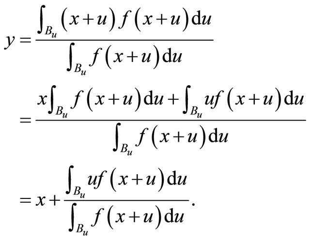
  , we define the search direction to be
 , where
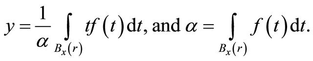 (2)
(2)
We also call y the local center of gravity of  in this paper. We prove that
  is a locally improving direction in the next Theorem.
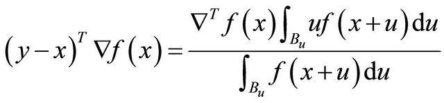
Theorem 2.1 The searching direction  satisfies
Especially, for a quadratic , we have
Proof. Let , and by definition of the local center of gravity,
 (3)
(3)
Hence
 (4)
(4)
Since ,
,  , and the sign of
  only depends on
 . In the following we first study
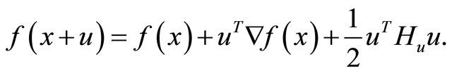
 . The second Taylor expansion of
  at x for sufficiently small u is
We note that  may change with u. For brevity, we also define
 .
.
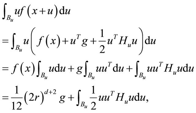 (5)
(5)
where the last equality used 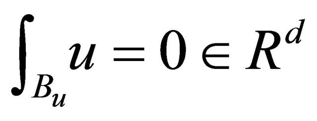 and
and
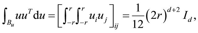
since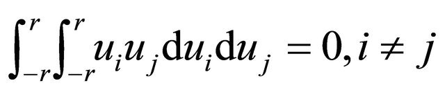 ,
,
 , and
, and .
.
 is the
  identity matrix.
For quadratic ,
,  , hence
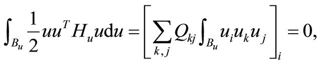
since  for all possible i, k, j combinations. Since
 , a maximum of
 ,
,  for all x in B exists. Hence
 (6)
(6)
Applying this result into (4),
when .
. 
Theorem 2.1 shows that the algorithm always generate an improving direction. Furthermore, the theorem shows that for a quadratic objective function, the integration based search direction is exactly the steepest descent direction. Though the analytical form of the objective function  is unknown, our closed form expression for quadratic case clearly indicates the capability of interation based searching direction, especially it is well known that sequential quadratic approximations of C2 function can be effective, which sheds lights on future research.
With the aboved establied improving feasible direction, we can directly apply the well established idea of feasible direction algorithm Theorem 10.2.7 [20]. The idea is fairly simple: given a feasible point , an improving feasible direction
  satisfying (1)
  is feasible, and (2) the objective value is better at
  for sufficiently small
 , a one dimensional optimization problem is solved to determine how far to proceed along
 , which leads to a new point
 , and the process is repeated.
Theorem 2.2 Let  be feasible,
  ,
,  obtained from (2),
  , where
  is optimal for the one dimensional optimization problem
 . Then the sequence
  converges to a KKT point.
Proof. See Theorem 10.2.7 [20]. 
While our convergence analysis can take benefit of the well established optimization theories; in the contrast, the convergence analysis of the directional direct search algorithm [8,9] relies on searching a predefined set of directions, which spans the searching space.
Our next example shows that when r is large, the searching direction generated by the algorithm is not necessary a locally improving direction. However, as the examples shows, it points to the global optimum.
Example 2.1 Let . Its second order Taylor expansion is
 ,
,
 , and
, and . It can be shown that
 (7)
(7)
We are not following the steps of (6) here since 
is known explicitly. For simplicity, let ,
,  ,
,
 ,
, . With this choice,
  on
on .
. , hence
  for
for .
.
For x in this range  leads to conclusion
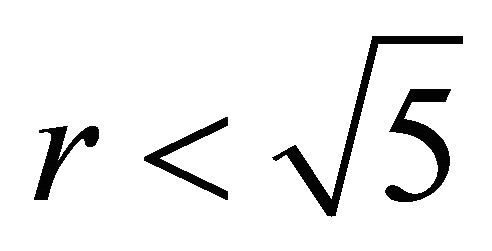 . The bound is sharp as we see that with
  the gradient is 1. If we choose
  within the bound, the center of gravity for this problem is
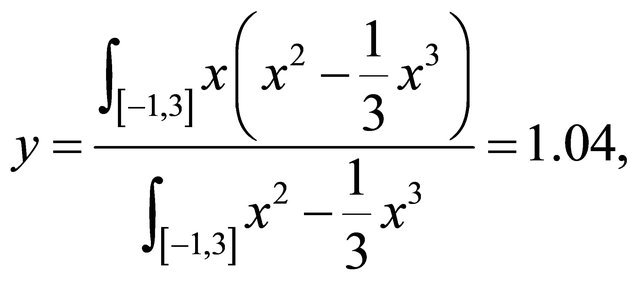
which is bigger than x = 1 and aligned with the gradient g. However, if we choose r = 3, then a similar calculation shows that the center of gravity on  is 0.85, which points to region with larger objective values than the local maximum.
It is not a surprise that when r is large, the algorithm is able to generate searching directions towards the global optimum, since more information of the function is used. In the contrast, a gradient only reflects the local structure of the function. This observation leads to our development of a new heuristic. We use large r at beginning of the algorithm with an intention to explore the overall structure of the objective function. This global probing phase ends when successive iterates are close enough to each other, which implies that two iterates are in the same hump. In the next phase, we would like the algorithm to find the maximum of this hump, hence we use a very small r and fast update to achieve the local convergence.
3. Starting Point
We know that the starting point is very important for a nonlinear optimization problem. We propose to use the center of gravity of  on B as the starting point. By its construction, the center of gravity tends to locate in a high valued neighbourhood, hence provides an effective starting point. In the following theorem, we show that this simple heuristic starting point strategy can always lead to a global optimum for the mixture model in statistics under some assumptions. This strategy is new and seems effective in our numerical experiments.
Theorem 3.1 Consider a statistical mixture model
 (8)
(8)
where  are density functions,
  ,
, . Without loss of generality, assume
 . Assume that the global optimum
  is unique and satisfies
 . Define
 where
where . If
. If  and
and
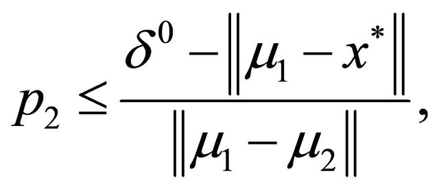 (9)
(9)
where 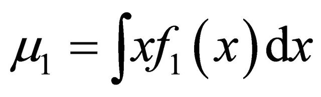 and
and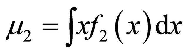 , then the algorithm converges to the global optimum if started from
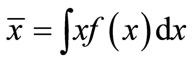 .
.
Proof. Observe that
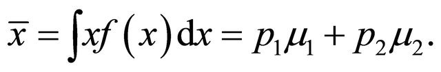 (10)
(10)
We then have
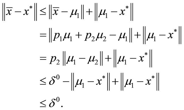
This implies that , hence the local improving directions leads to
  if
if .
. 
We remark that the above result is applicable to a broader functional class with proper normalization. For a composite function
 (11)
(11)
where  are non-constant and nonnegative functions, it can be normalized as
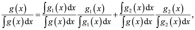
which is precisely the mixture form  with
with
The condition,  implies that
  This implies that
  makes larger contribution to the total integration than
 .
.
4. Sparse Grid Numerical Integration
Since the algorithm relies on the numerical integration to calculate the local center of a gravity at each step and the starting point, its accuracy and efficiency is crucial to the success of our algorithm. We integrate the modern sparse grid method [21] into our algorithm. In this section, we first briefly introduce the sparse grid method. Then we present our result on this aspect: a new closed form formula for the number of function calls used in the sparse grid numerical integration. The complexity of sparse grid method itself has been studied by various authors, and the order of complexity is shown in [19]. Our result makes it explicit how many function calls are used exactly in the integration step in our algorithm. Since the sparse grid method itself is not our contribution, our introduction is terse for the purpose of explaining the necessary notations used in our derivation of the closed form formula. For details of the sparse grid method, we refer our readers to [22].
Numerical integration for univariate function (quadrature) uses the weighted sum of function values as the approximation to the integration:
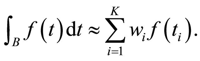 (12)
(12)
A central problem in quadrature is to decide the weights  and grid points
 . In this sense, GaussLegender quadrature uses an optimal solution to the following optimization problem:
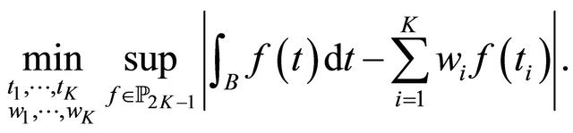 (13)
(13)
Clearly the model minimizes the worst case approximation error for any univariate polynomial function with order up to . Different univariate quadrature rules have been derived.
Extension of univariate quadrature to multivariate quadrature is difficult due to the curse of dimensionality. Among various approaches, the sparse grid method uses an interesting tensor product of univariate quadratures. In the following we first outline necessary details of this tensor product, on which our analysis of number of function evaluations is based on.
We define an operator :
:
 (14)
(14)
where  specifies the set of evaluation points, and
  provides the corresponding weights. We note that for Gauss-Legender univariate quadrature, the cardinalities for
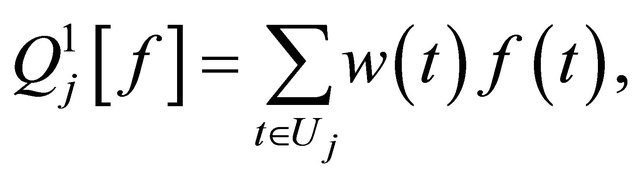
 . We define a difference operator as:
Clearly the difference operator  is defined on the point set
 , and it could also be represented as a weighted sum of function values:
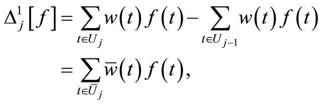
where the weight function 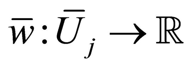 could be calculated mechanically. We define the tensor product of difference operator as
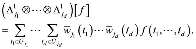 (15)
(15)
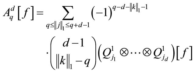
The sparse grid approach (Smolyak 1960) extends the univariate quadrature  to the multivariate quadrature rule
  (via the intermediate difference operator
 ) as for
 :
:
 (16)
(16)
 has no approximation error [23] for polynomials in the space
 ,
,  , if each univariate quadrature rule
  has no approximation error for the univariate polynomial space
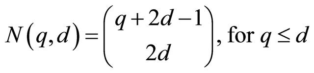
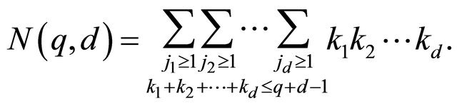
 . For smooth functions, not necessarily polynomial, the sparse grid method also achieves high accuracy [19]. Also see [22] for spare grid implementation details. In this paper, the most relevant question is how many function calls are used in a sparse grid numerical integration. Though the order of magnitude of this number is known, see Lemma 3.6 in [21] and [22], we derive a new and exact formula. The exact formula shows that the number of function calls in computing the local center of gravity is
 .
.
Proposition 4.1 Using the Gauss-Legender sparse grid rule , Subroutine 2 makes
  function calls.
Proof: Applying Theorem 4.1 for the special case .
.
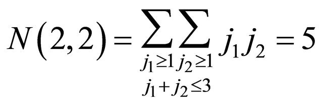
Theorem 4.1 The Gauss-Legender sparse grid rule  uses
uses  function calls, where
 (17)
(17)
Furthermore,
 (18)
(18)
Proof. For the Gauss-Legender univariate rule , the number of points is
 , and
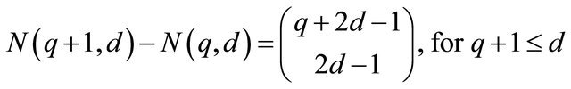
, and . Furthermore, [23] shows that (combination rule):
 (19)
(19)
Hence for ,
,
 (20)
(20)
1) The closed formula (17) apparently holds for  and
and  since
since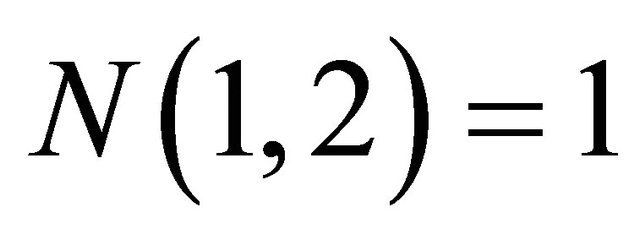 , and
, and
2) Assume the formula (17) is valid for d and . We now consider the case for
 .
.
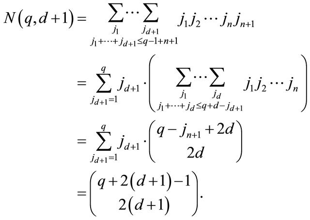
The last step
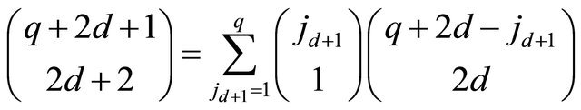 (21)
(21)
can be proved by the following equivalence: selections of  balls out of
  identical white balls is equivalent to: choose one ball from the first
  balls and there are
  ways; choose the
ball as the second ball and color it red; choose 2d balls from the rest and there are  ways. Total number of balls before the red could be one to q. The maximal number is q since otherwise there is less than 2d balls behind the red.
3) Hence the formula (17) is valid by mathematical induction.
The second half of the theorem follows this identity

5. Algorithm
Algorithm 1 Sparse Grid Derivative Free Algorithm (SGDF)
1: global probing phase:
2: , see Subroutine 2 3:
4: repeat 5: 
6: 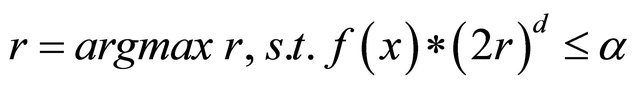 ,
, 
7: 
8:  , see Subroutine 2 9: linesearch along y − x to get z, see Subroutine 3 10: until
11: local convergent phase:
12: repeat 13: 
14: steps (4)-(10)
15: until
As shown in Algorithm 1, it has two phases: the global probing phase and the convergent phase. The two phases differs only in the parameter , and are identical otherwise. In the global probing phase,
  constantly; while in the convergent phase
 . Both phases share same iteration steps (4)-(10), which are essentially numerical implementation of (2) with line search for additional efficiency. In the global phasing phase, the algorithm uses 90% terrain of the feasible region to determine the search direction. This provides great opportunity for the algorithm to escape from local optimum traps. When two successive iterates
  and
and  are very close, we switch to the convergent phase, where we exponentially decay
 . By focusing on a less portion of the terrain, the algorithm is able to advance to a local optimum accurately. Details of one iteration is the follows. We first approximate the radius for the given
  through mid-point quadrature rule in the step 6. The new domain
  is defined in the step 7. Step 8 computes the center of gravity of the new domain
  using the subroutine 2. Step 9 conducts a linear search subroutine 3 to accelerate the algorithm.
The subroutine 2 computes the center of gravity (cg), which calls the sparse grid algorithm in its first step to generate n sparse grid points as briefly introduced in section 4. In our numerical implementation, we called the public domain Matlab package Sparse Grid Toolbox by Andreas Klimke. We note that each numerical integration uses only  function calls as proved in the Proposition 4.1. In the subroutine 2, the volume of the domain
  is computed in the step 3 and is used in lieu in the following step 4. We also point out that function evaluations at grid points are computed in step (2) only once. These values are stored and used later in steps (3) and (4).
Subroutine 2: Center of gravity 
1: Generate n sparse grid points  of the given rectangle
 , see Section 4 2: Compute
3: Compute the volume 
4: Compute 
In the subroutine 3 we equip a special derivative free line search for SGDF enhance its numerical efficiency. The idea is to move along the line  as much as possible. We observe that it is often too conservative to move to
  only; instead, search along the line often brings huge performance gain. The line search is greedy: it moves forward by a fixed stepsize until the function value is worse or it hits the boundary; then it bisects the stepsize and retreats a stepsize until it finds the first feasible and improving point or until the stepsize is less than
 .
. ,
,  ,
,  are all set at
  level.
Subroutine 3: Derivative free line search
Ensure: ;
;
1: initialize ;
;
2: while  and
and  is feasible do 3:
4: end while 5: repeat 6: 
7: until  is feasible and either
  or
or 
8: return 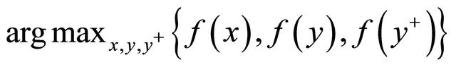
6. Numerical Tests
We compare SGDF with the state-of-art derivative free algorithms, including Pattern Search or Direct Search (with and without poll step) [24], Global Search [25], Multi-start [26], Simulated Annealing and Genetic algorithm [27]. These algorithms have mature industrial strength implementations in MATLAB Global Optimization Toolbox. We also implemented our new SGDF algorithm in MATLAB and conducted comparative study.
We use their default settings for the solvers from the Matlab Global Optimization Toolbox. Pattern Search Algorithm uses only poll step by default. However, it is more efficient when coupled with a searching step. Hence we compare with the Pattern Search algorithms with and without the searching option. Both the Global Search Solver and the Multistart Solver needs a local solver. We followed the recommendation from Matlab manual and set the Interior-Point-Method as local solver for the Global Search, and the medium scale algorithmic option for the Multistart.
In contrast to the SGDF deterministic starting point strategy, all these derivative free algorithms rely on random starting points or user inputs. Global Search uses a scatter-search mechanism [26] for generating random start points. MultiStart uses uniformly distributed start points within bounds (default 10), or user-supplied starting points. Global Search analyzes starting points and rejects those points that are unlikely to improve the best local minimum found so far. In the contrast, a MultiStart solver runs the local solver from all feasible starting points.
Since these algorithms use random starting points, a single run result could be very poor or excellent. To get a whole picture, we run each solver 26 times (arbitrarily chosen) and use the median number of failures as a measure of its accuracy measure. A run fails if its error exceeds 5% in terms of the objective value:
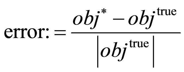 (22)
(22)
We use the number of function calls as efficiency measure. This is a convention in testing derivative free algorithms since function evaluations are expensive for typical derivative free optimization problems. On the other side, for the purpose of constructing searching directions, Newton and other high order methods spend a significant amount of time on inverting matrix or solving equations; while derivative free algorithms typically don’t involve this overhead. Their expense in constructing search directions can also be reasonably measured in number of function evaluations. For SGDF, this expense is on the numerical integration. For other derivative free algorithms, this expense is also on point-wise evaluation based interpolation, pseudo differentiation or simplex derivatives. Again, due to the random starting strategy employed by other derivative free algorithms, we use the median number of function calls of their 26 runs as a robust measure of their efficiency.
We use eight test functions [28]: Brianin, Six-Hump, Goldstein Price, Hartman3, Hartman6, Shekel5, Shekel7, and Shekel10. These functions have known optimal values and optimal solutions, and have been used widely for testing purpose in research papers. For these functions, their dimensions and known optimal values are tabulated in the Table 1. We also show the optimal values from SGDF side-by-side with the true optimal value in Table 1, which clearly shows that SGDF is capable of achieving high accurate results.
Table 2 shows number of failures for each algorithm as a measure of accuracy. SGDF has no failure, which is also achieved by MS. All other algorithms have difficulty for high dimensional problems. Especially the genetic algorithm and pattern search without polling option exhibit high failure rates.The multi-start strategy (MS), though simple, works very well. SGDF, on the other hand, uses a more complicated strategy. It uses global information of the objective function in the global probing phase, and generates searching directions pointing to region with high objective values on average. This searching heuristics is fundamentally different from the local searching idea. Apparently, this innovative searching heuristics can also be coupled with the simple multistart idea to enhance its success rate. However, multistart inherently increases the computation effort as seen in the next table. Hence how to efficiently combine strength from both methods is a subject of future research.
Table 3 shows the median number of function calls used by each algorithm as a measure of efficiency. It is clear that SGDF uses much less function calls than multistart algorithm. A further calculation shows that SGDF uses 65% less function calls than multi-start algorithm. This is not a surprise since multi-start algorithm runs from ten starting points so as to increase its chance of hitting the global. Global Search also uses multiple starting points, but it drops those unpromising ones sooner. However, Global Search does not simply run local solver from each starting point, it has a more complicated strategies including basin radius estimation, two stage search, and dynamic threshold, etc, which increases its function calls significantly. Pattern Search with additional searching option is more efficient than Pattern
Table 1. Compare the true and SGDF optimal objective values.
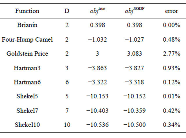
Table 2. Median number of failures.
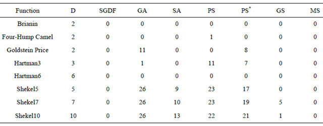
SGDF: sparse grid derivative free; GA: genetic; SA: simulated annealing; PS: pattern search (direct search); PS*: pattern search with polling option on; GS: global search; MS: multi-start.
Table 3. Median number of function calls.
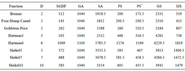
SGDF: sparse grid derivative free; GA: genetic; SA: simulated annealing; PS: pattern search (direct search); PS*: pattern search with polling option on; GS: global search; MS: multi-start.
Search with polling step only. Simulated Annealing and Genetic algorithms apparently use more function calls.
Tables 2 and 3 together show that SGDF is both accurate and efficient. Multi-start is accurate but slightly more expensive. Global Search and Simulated Annealing could be accurate at the expense of more than ten times function calls as SGDF. The Pattern Search with or without searching step is efficient, but could generate a solution far away from optimum if started randomly. Genetic algorithm has reported success for more complicated biological system optimization but does not advantage in this experiment.
It appears that the starting point strategy of SGDF is effective. By using a single starting point, i.e., the global center of gravity, SGDF is able to find solutions very close to a global optimum for eight testing problems. In the contrast, other algorithms use random starting points have more or less fails, except for multi-start algorithm. The multi-start algorithm uses ten starting points in each of the twenty six runs. It is interesting to observe that for this experiment there is always one good starting point out of the ten.
7. Conclusions and Discussion
In this paper, we present a new integration based derivative-free optimization algorithm. The new idea of using integration to generated searching direction has its advantages: we prove that when the integration area is small, the generated direction is always an improving one; we also demonstrate that by simply enlarging the integration area, the algorithm can make use of global information, and generate a searching direction towards area with high objective values on average. We also propose an innovative starting point strategy based on integration. We not only use the modern sparse grid method to implement the integration, but also make contribution in the sparse grid method theory, as we see the need in accurately counting the number of function calls. The new algorithm is also clearly structured in two phases: a global probing phase and a local convergence phase. We equip a new derivative free robust line search method for the algorithm as well. Computational experiments clearly shows that the new heuristic algorithm is accurate and efficient. The result of benchmarking against state-of-art derivative free optimization methods, including Pattern Search, Global Search, Multi-start, Simulated Annealing and Genetic algorithms, is favorable.
The new algorithm is intended to solve practical problems, where derivative information is not available and function evaluation is expensive. For these problems, priority is given to generate a high quality near-optimal solutions within computing budget. On the other hand, we realize that many of these problems also involve integer decision variables, which is not handled by the current algorithm, hence it is a topic for our future research.
REFERENCES
- J. D. Pinter, “Global Optimization in Action,” Kluwer, Dordrecht, 1996. doi:10.1007/978-1-4757-2502-5
- A. J. Booker, J. E. Dennis Jr., P. D. Frank, D. W. Moore and D. B. Serafini, “Managing Surrogate Objectives to Optimize a Helicopter Rotor Design: Further Experiments,” Proceedings of 8th AIAA/ISSMO Symposium on Multidisciplinary Analysis and Optimization, St. Louis, 1998.
- C. Audet and D. Orban, “Finding Optimal Algorithmic Parameters Using Derivative-Free Optimization,” SIAM Journal on Optimization, Vol. 17, No. 3, 2006, pp. 642- 664.
- R. Oeuvary and M. Bierlaire, “A New Derivative-Free Algorithm for the Medical Image Registration Problem,” International Journal of Modelling and Simulation, Vol. 27, No. 2, 2007, pp. 115-124.
- T. Levina, Y. Levin, J. Mcgill and M. Nediak, “Dynamic Pricing with Online Learning and Strategic Consumers: An Application of the Aggregation Algorithm,” Operations Research, Vol. 57, No. 2, 2009, pp. 327-341.
- P. Mugunthan, C. A. Showmaker and R. G. Regis, “Comparison of Function Approximation, Heuristic and Derivative-Based Methods for Automatic Calibration of Computationally Expensive Groundwater Bioremediation Models,” Water Resources, Vol. 41, 2005.
- J. A. Neldder and R. Mead, “A Simplex Method for Function Minimization,” The Computer Journal, Vol. 7, No. 4, 1965, pp. 308-313. doi:10.1093/comjnl/7.4.308
- C. Audet and J. E. dennis Jr., “Analysis of Generalized Pattern Searches,” SIAM Journal on Optimization, Vol. 13, No. 3, 2003, pp. 889-903. doi:10.1137/S1052623400378742
- T. G. Kolda, R. M. Lewis and V. Torczon, “Optimization by Direct Search: New Perspectives on Some Classical and Modern Methods,” SIAM Review, Vol. 45, No. 3, 2003, pp. 385-482. doi:10.1137/S003614450242889
- T. A. Winslow, R. J. Trew, P. Gilmore and C. T. Kelley. “Doping Profiles for Optimum Class B Performance of GaAs MESFET Amplifiers,” Proceedings of the IEEE/ Cornell Conference on Advanced Concepts in High Speed Devices and Circuits, Ithaca, 5-7 August 1991, pp. 188- 197.
- A. R. Conn, K. Scheinberg and P. L. Toint, “On the Convergence of Derivative-Free Methods for Unconstrained Optimization,” Approximation Theory and Optimization: Tributes to M. J. D. Powell, Cambridge University Press, Cambridge, 1997, pp. 83-108.
- M. J. D. Powell, “The NEWUOA Software for Unconstrained Optimization without Derivatives,” Technical Report, DAMTP 2004/NA08, Department of Applied Mathematics and Theoretical Physics, University of Cambridge, Cambridge, 2004.
- M. Marazzi and J. Nocedal, “Wedge Trust Region Methods for Derivative Free Optimization,” Mathematical Programming, Vol. 91, No. 2, 2002, pp. 289-305. doi:10.1007/s101070100264
- A. R. Conn, K. Scheinberg and L. N. Vicent, “Introduction to Derivative-Free Optimization,” MOS-SIAM Series on Optimization, SIAM, Philadelphia, 2009. doi:10.1137/1.9780898718768
- C. Audet and J. E. Dennis Jr., “Mesh Adaptive Direct Search Algorithms for Constrained Optimization,” SIAM Journal on Optimization, Vol. 17, No. 1, 2006, pp. 188- 217. doi:10.1137/040603371
- D. Jones, C. Perttunen and B. Stuckman, “Lipschitzian Optimization without the Lipschitz Constant,” Journal of Optimization Theory Applications, Vol. 79, No. 1, 1993, pp. 157-181, doi:10.1007/BF00941892
- W. Huyer and A. Neumaier, “Global Optimization by Multileve Coordinate Search,” Journal of Global Optimization, Vol. 14, No. 4, 1999, pp. 331-355. doi:10.1023/A:1008382309369
- X. Wang, D. Liang, X. Feng and L. Ye, “A DerivativeFree Optimization Algorithm Based on Conditional Moments,” Journal of Mathematical Analysis and Applications, Vol. 331, No. 2, 2006, pp. 1337-1360.
- G. W. Wasilkowsi and H. Wozniakowski, “Explicit Cost Bounds of Algorithms for Multivariate Tensor Product problems,” Journal of Complexity, Vol. 11, No. 1, 1995, pp. 1-56. doi:10.1006/jcom.1995.1001
- M. S. Bazarra, H. D. Sherali and C. M. Shetty, “Nonlinear Programming: Theory and Algorithms,” 3rd Edition, Wiley, John & Sons, Hoboken, 2006.
- H.-J. Bungartz and M. Griebel, “Sparse Grids,” Acta Numerica, Vol. 13, 2004, pp. 147-269.
- T. Gerstner and M. Griebel, “Numerical Integration Using Sparse Grid,” Numerical Algorithms, Vol. 18, 1998, pp. 209-232.
- F.-J. Delvos, “D-Variate Boolean Interpolation,” Journal of Approximation Theory, Vol. 34, No. 2, 1982, pp. 99- 114. doi:10.1016/0021-9045(82)90085-5
- A. R. Conn, N. I. M. Gould and P. L. Toint, “Trust-Region Methods,” MOS-SIAM Series on Optimization, SIAM, Philadelphia, 2000. doi:10.1137/1.9780898719857
- Z. Ugray, L. Lasdon, J. Plummer, F. Glover, J. Kelly and R. Marti, “Scatter Search and Local NLP Solvers: A Multistart Framework for Global Optimization,” INFORMS Journal on Computing, Vol. 19, No. 3, 2007, pp. 328-340. doi:10.1287/ijoc.1060.0175
- F. Glover, “A Template for Scatter Search and Path Relinking,” In: J.-K. Hao, E. Lutton, E. Ronald, M. Schoenauer and D.Snyers, Eds., Artificial Intelligence, Springer, Berlin, Heidelberg, 1998, pp. 13-54.
- D. E. Goldberg, “Genetic Algorithms in Search,” Optimization & Machine Learning, Addison-Wesley, Boston, 1989.
- L. C. W. Dixon and G. P. Szegö, “The Global Optimization Problem: An Introduction,” Towards Global Optimisation 2, North-Holland Pub. Co, Amsterdam, 1978, pp. 1-15.