Journal of Encapsulation and Adsorption Sciences
Vol.3 No.3(2013), Article ID:37166,16 pages DOI:10.4236/jeas.2013.33010
On Single Compartment Pharmacokinetic Model Systems That Obey Free Radical Copolymerization Kinetics and Multiplicity
Advanced Technology, Lone Star College-North Harris, Houston, USA
Email: jyoti_kalpika@yahoo.com
Copyright © 2013 Kal Renganathan Sharma. This is an open access article distributed under the Creative Commons Attribution License, which permits unrestricted use, distribution, and reproduction in any medium, provided the original work is properly cited.
Received April 25, 2013; revised May 25, 2013; accepted June 3, 2013
Keywords: Single Compartment Pharmacokinetics; Copolymer Composition; Reactivity Ratios; Multiplicity; State Space Model; n Monomers
ABSTRACT
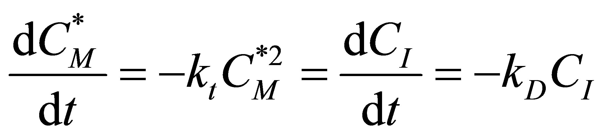
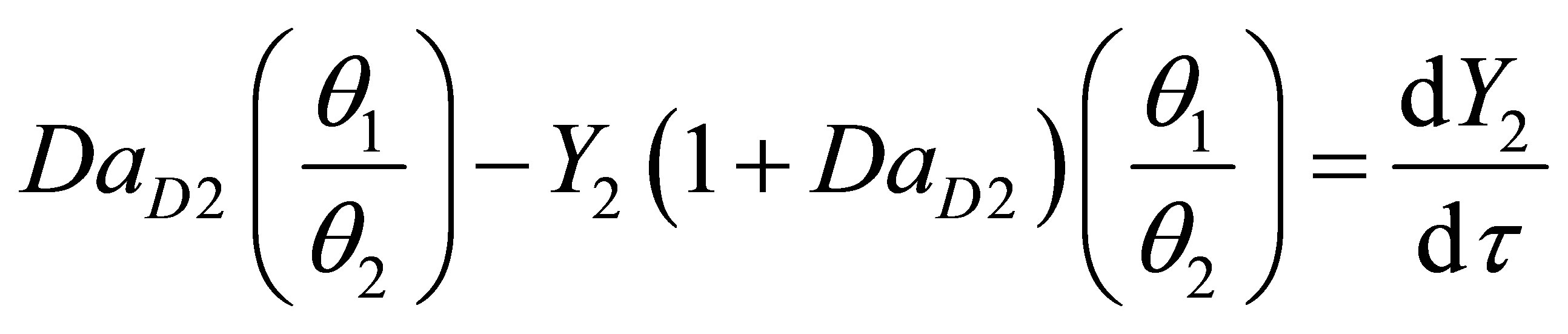
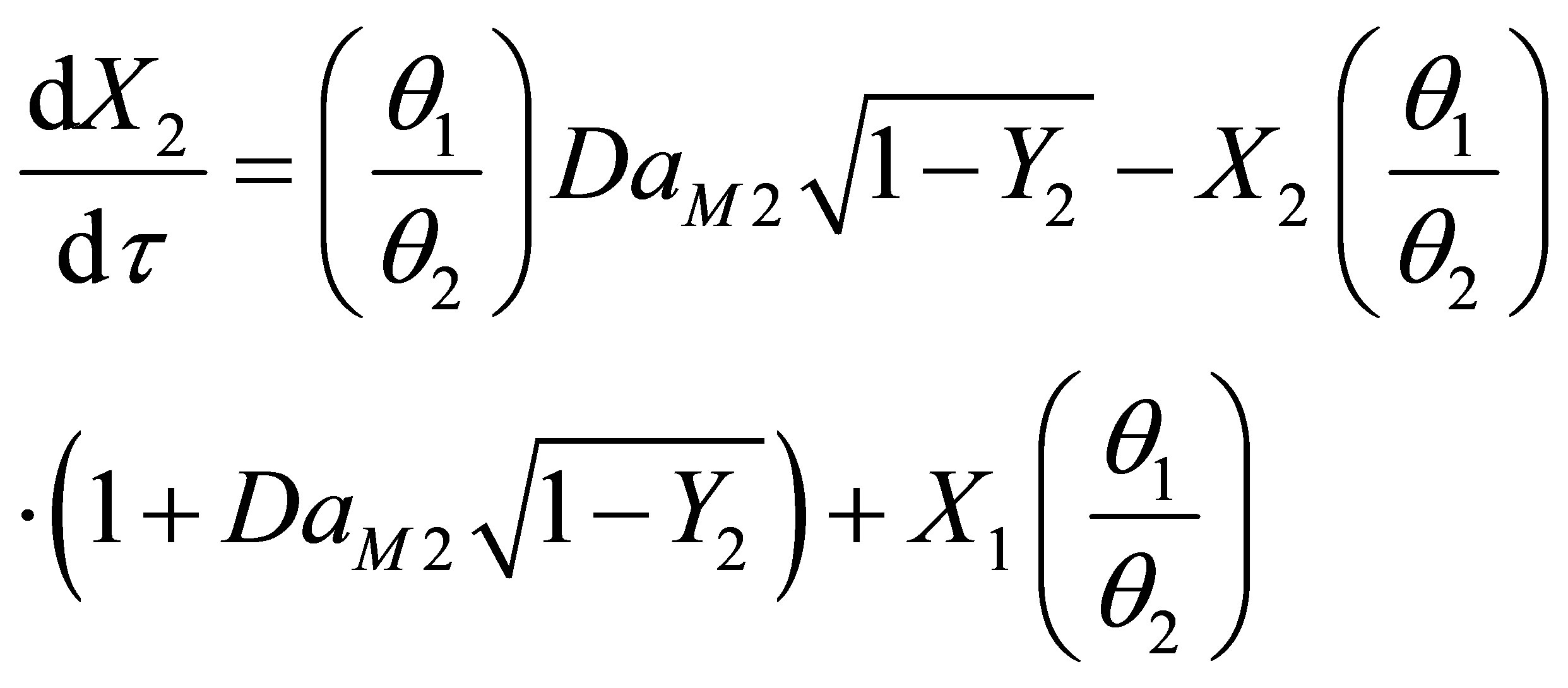
This study examines the issues in development of pharmacokinetic single compartment model for systems that obey free radical copolymerization kinetics. Copolymer composition as a function of reactivity ratios of comonomers for well mixed case was derived. For some cases, such as DEF-AN, diethyl fumarate and acrylonitrile system multiplicity in composition were found. The analysis is extended to n monomers. State space model expressions are used and the QSSA assumption is stated in state space equation form. Conditions when damped oscillations can be expected are noted. In addition to multiplicity in product composition, an account of reactivity ratios and other instances of multiplicity were found during the pharmacodynamics of the free radical polymerization reactions. A careful study of initiated case, thermal case, 1 CSTR and 2 CSTRS was undertaken and results were presented. Numerical integration techniques were employed on the desktop computer. Steady state and transient state conversion for initiated case and thermal case for 1 CSTR and 2 CSTRs were calculated and plotted in Figures 7-9 and 12. No multiplicity was found in the thermal case for 1 CSTR in the dynamics of transient monomer conversion. Multiplicity was found in the initiated case for 1 CSTR in the dynamics of transient conversion of monomer. The multiplicity was found in the second CSTR for the case of 2 CSTRs in series. No multiplicity was found in the case of initiator decay.
1. Introduction
Pharmacokinetics is the experimental, theoretical and computational analysis of rate of change with time of concentration and volume distribution of compounds administered externally such as drugs, metabolite, nutriaents, harmones and toxins, all in various regions of the human physiology [1,2]. Application of pharmacokinetics allows the processes of liberation, absorption, distribution, metabolism and excretion to be characterized mathematically. The absorption of drug can be affected by different methods. Drugs administered through the gastrointestinal tract, which is referred to as enteral route of entry. Parenteral routes refer to all other types of drug entry drug administration:
1) Sublingual Entry—beneath the tongue 2) Buccal Cavity—via the mouth 3) Gastric Entry—through stomach 4) IV Therapy—through veins 5) Intra muscular Therapy—with/in the muscular 6) Sub-cutaneous Therapy—beneath the epidermal and dermal skin layers 7) Intradermal Therapy—within the dermis 8) Percutaneous therapy—by topical treatment applied to the skin 9) Through mouth, nose, pharynz, trachea, bron-chi, bronchioles, alveolar sacs, alveoli by inhalation;
10) Intra arterial route—introduced into artery 11) Intrathecal Route—to cere-brospinal fluid 12) Vaginal Route—within the vagina 13) Itraocular Route—through eye 14) Systemic circulation is reached by the drugs absorbed from the buccal cavity and the lower rectum Pharmacokinetics is modeled using compartment models. Compartmental methods [1] involve development of mathematical models to describe the change in concentration of drug with time. These models are similar to those developed in chemical reaction engineering thermodynamics and biochemical kinetics. Compartmental models offer the advantage of prediction of drug concentration at any instant of time. There is a spectrum of pharmacokinetic model and computer software ranging from a simple one-compartmental pharmacokinetic mode with bolus administration with elimination to complex models that rely on the use of physiological information to ease development and validation. Although there are a number of discussions in the literature about pharmacokinetic models, most of them deal with monotonic exponential decay of concentration. Very little attention is paid to systems such as found during free readical polymerization of copolymers. This study deals with application of single compartment model pharmacokinetic analysis to systems that obey free radical copolymerization kinetics.
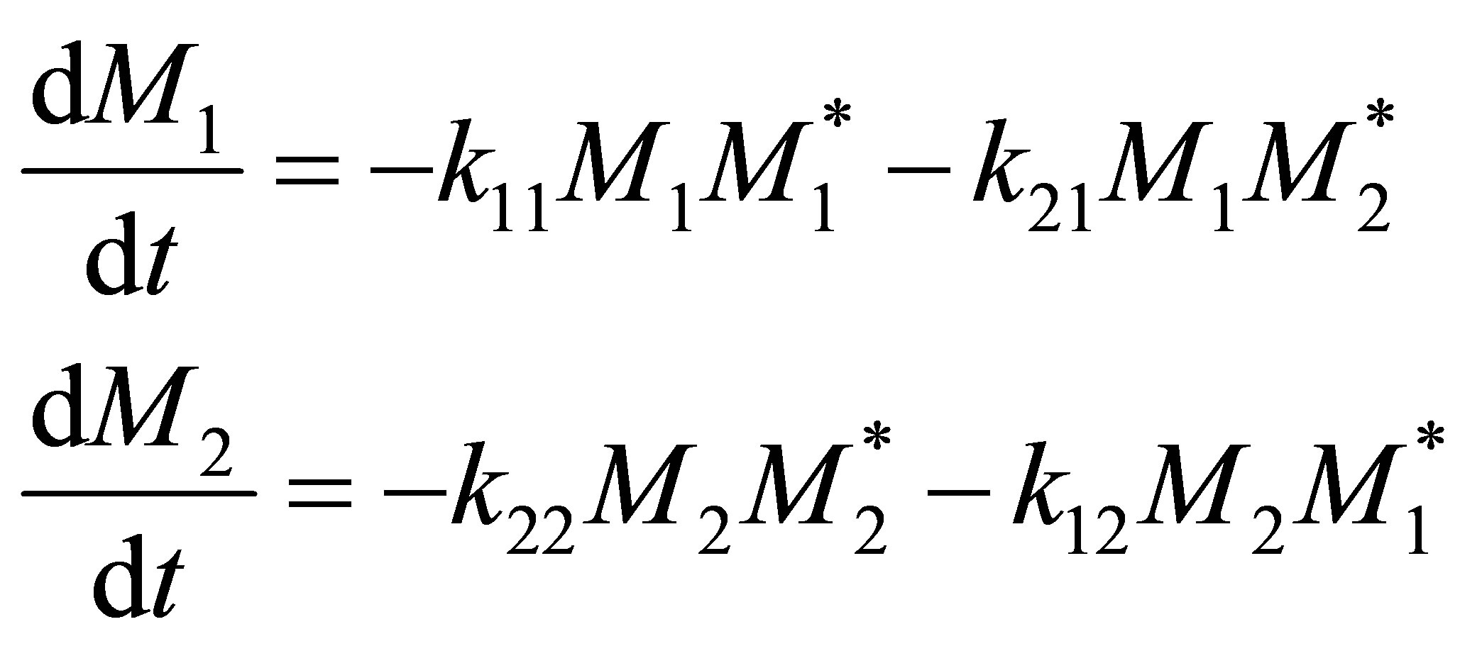
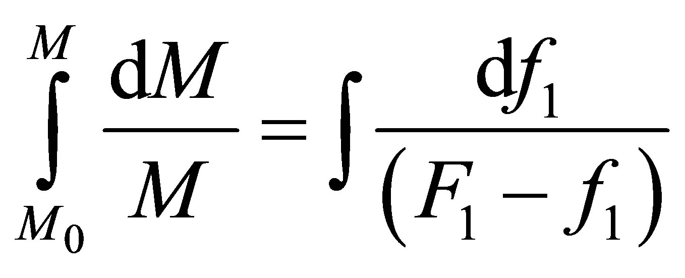
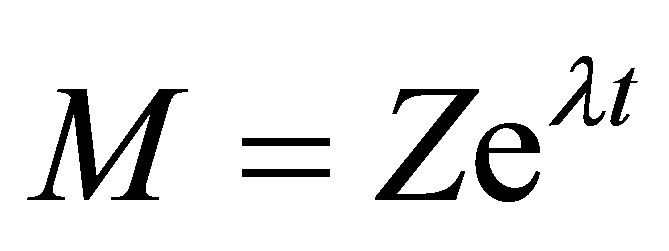
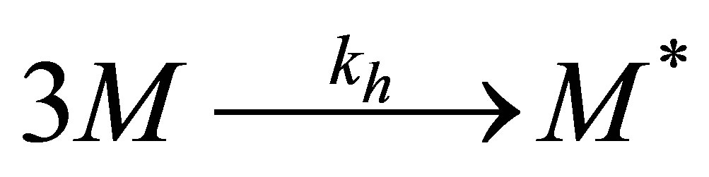
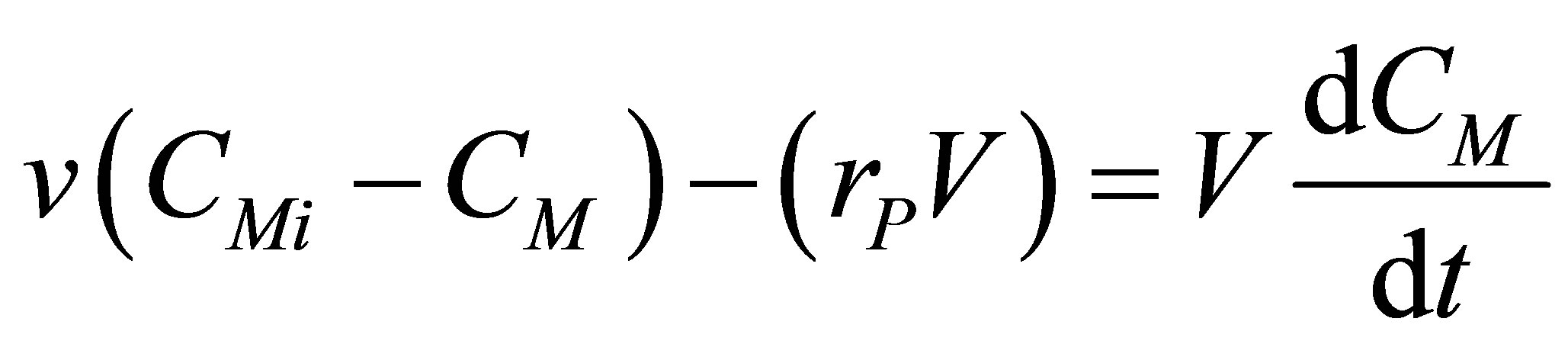
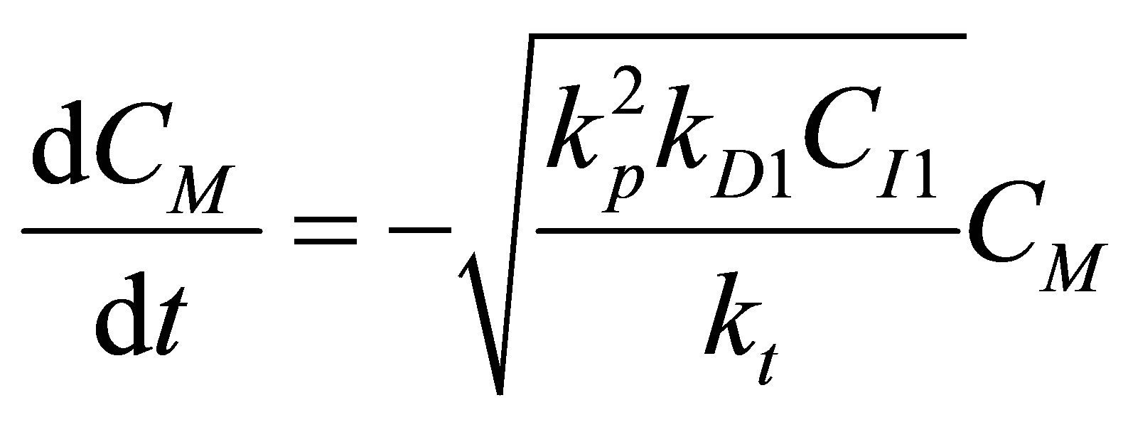
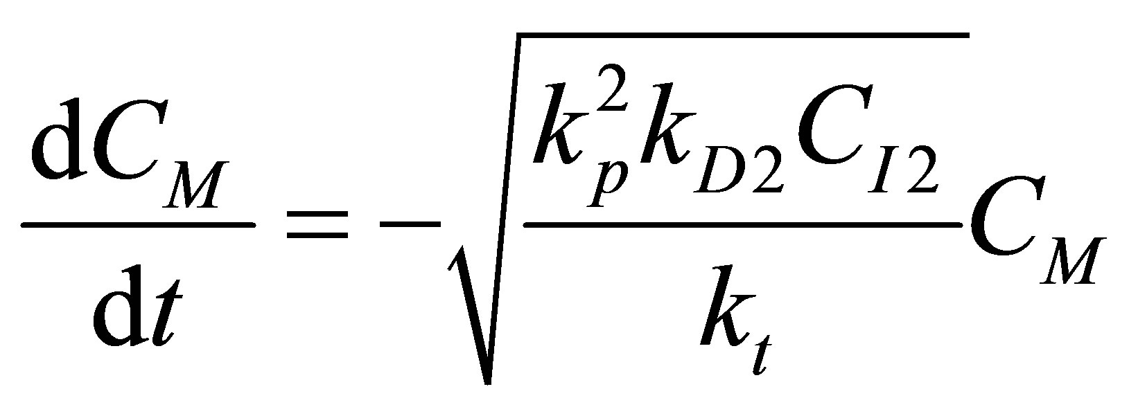
A mass balance on the concentration of drug within the human anatomy for the case where the kinetics of absorption is in obeyance of free radical copolymerizetion kinetics with elimination can be written for Figure 1 as: (1) Let M be the amount of drug that is available for absorption in comonomer form. The absorption of the drug process can be described by free radical copolymerization kinetics:
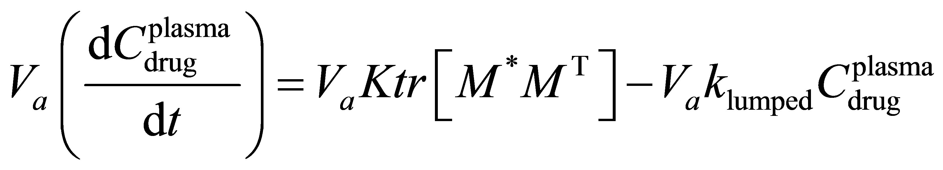 (1)
(1)
 (2)
(2)
2. Background
Multi-component copolymerization is a process by which two or more monomer repeat units enter the backbone chain of the polymer. This is different from polymers such as PET, polyethylene terephthalate or PA polyamide where the product is obtained by condensation polymerization. In the case of PET two starting materials, i.e., terepthalic acid and monoethylene glycol are reacted and water groups removed in the kettle in order to form the PET polymer backbone. Hexamethylene diamine and adipic acid go into the preparation of polyhexamethylene adipamide or nylon. Homopolymers are formed by chain polymerization of one monomer into polymer. With a
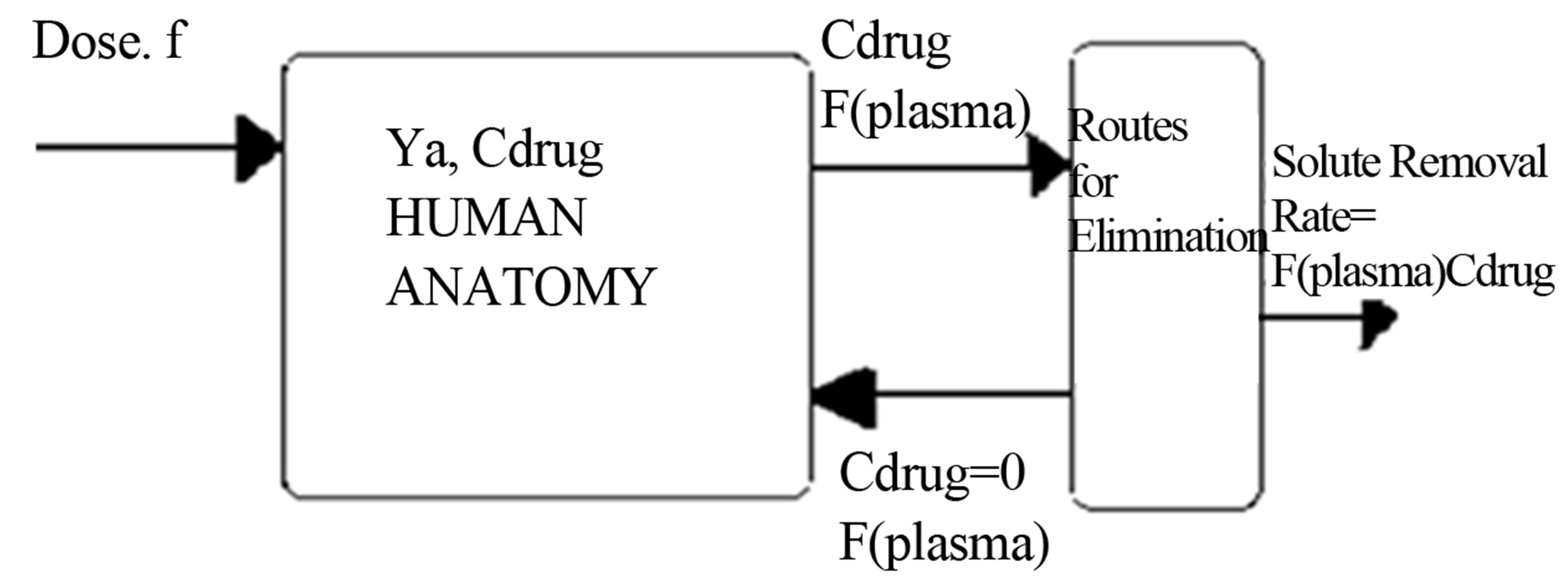
Figure 1. Single compartment model for human anatomy.
single monomer as the starting material with the repeat unit in the homopolymer, and the molecular weight is built by free radical reactions such as initiation, propagation and termination. Rather than one monomer when 2 or more monomers are pumped into the kettle, the polymer is found to have repeat units from the 2 or more monomers. This kind of product is called as copolymer. When more than 2 monomers are used, the term multicomponent copolymer may be used.
3. Composition of Random Copolymers
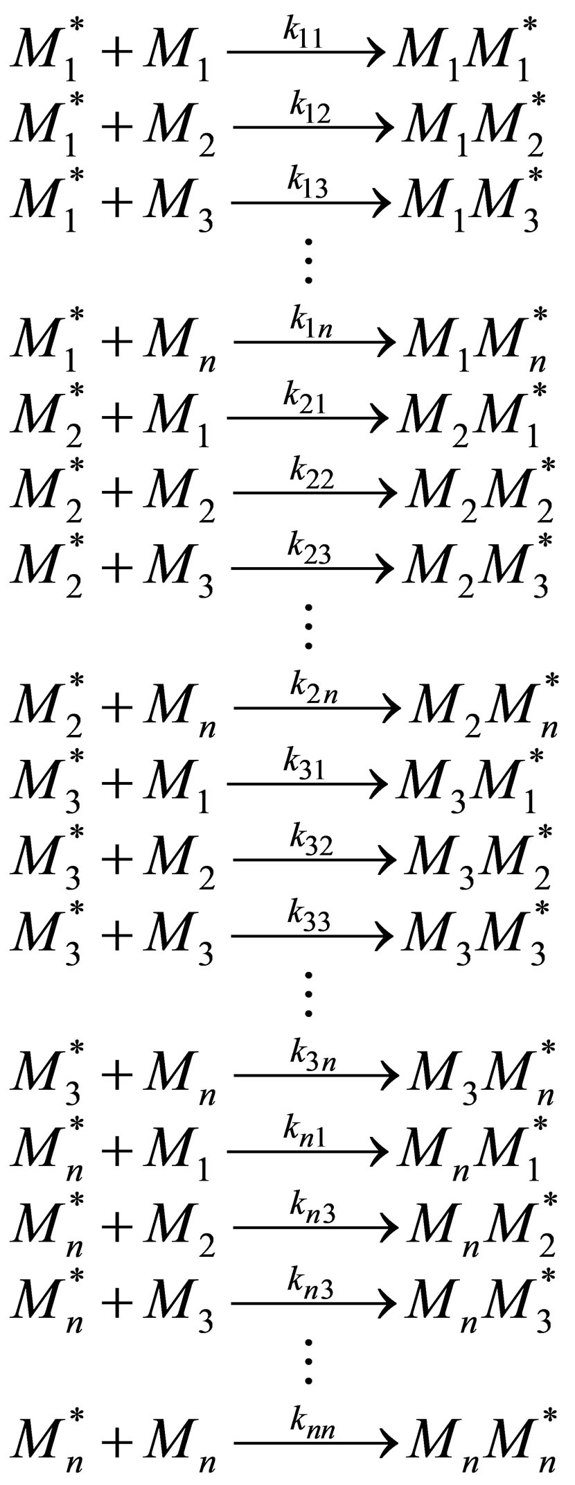
Copolymer composition can be calculated as a function of monomer composition when the polymer is formed by free radical polymerization in a CSTR (continuous stirred tank reactor). Consider two monomers 1 and 2 as starting materials for forming a copolymer with repeat units of 1 and 2. The initiation can be effected by thermal means or by using a peroxy initiator. The propagation reactions can be of four kinds:
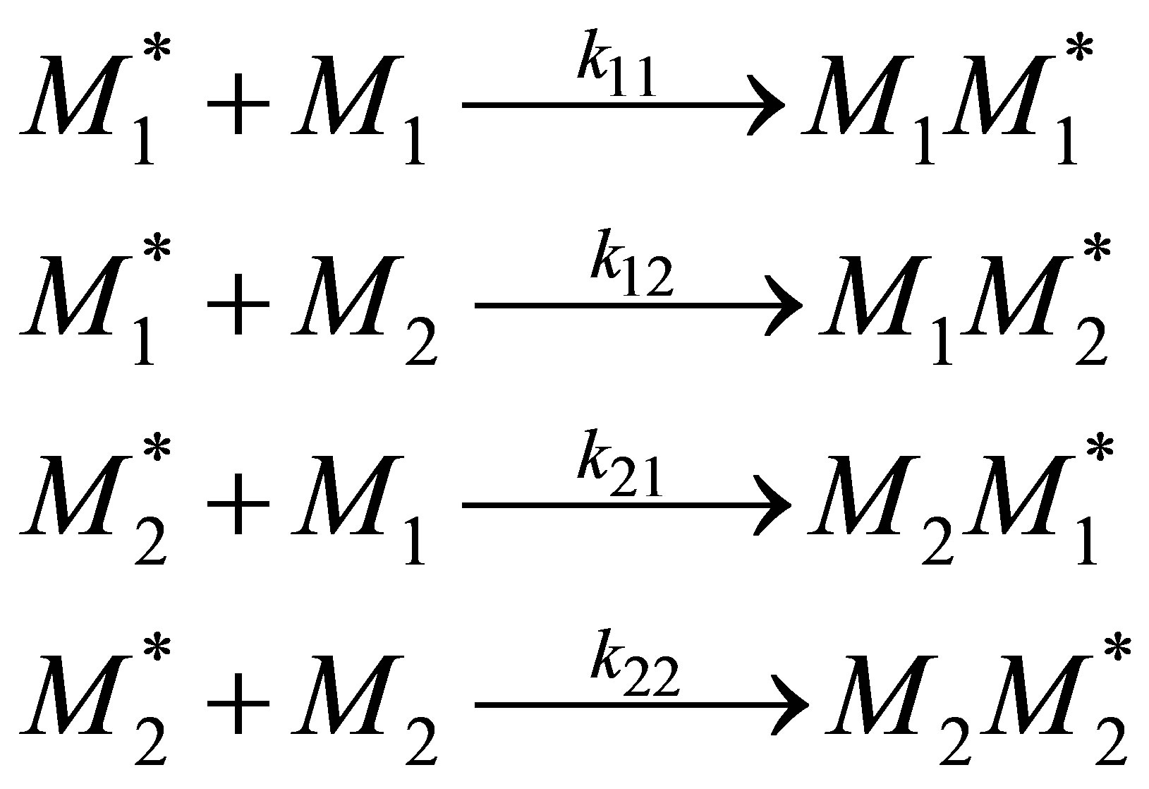 (3)
(3)
The rate of irreversible reactions can be written as follows:
 (4)
(4)
The free radical species formed may be assumed to be highly reactive and can be assumed to be consumed as rapidly as formed. This is the QSSA, quasi-steady state assumption.
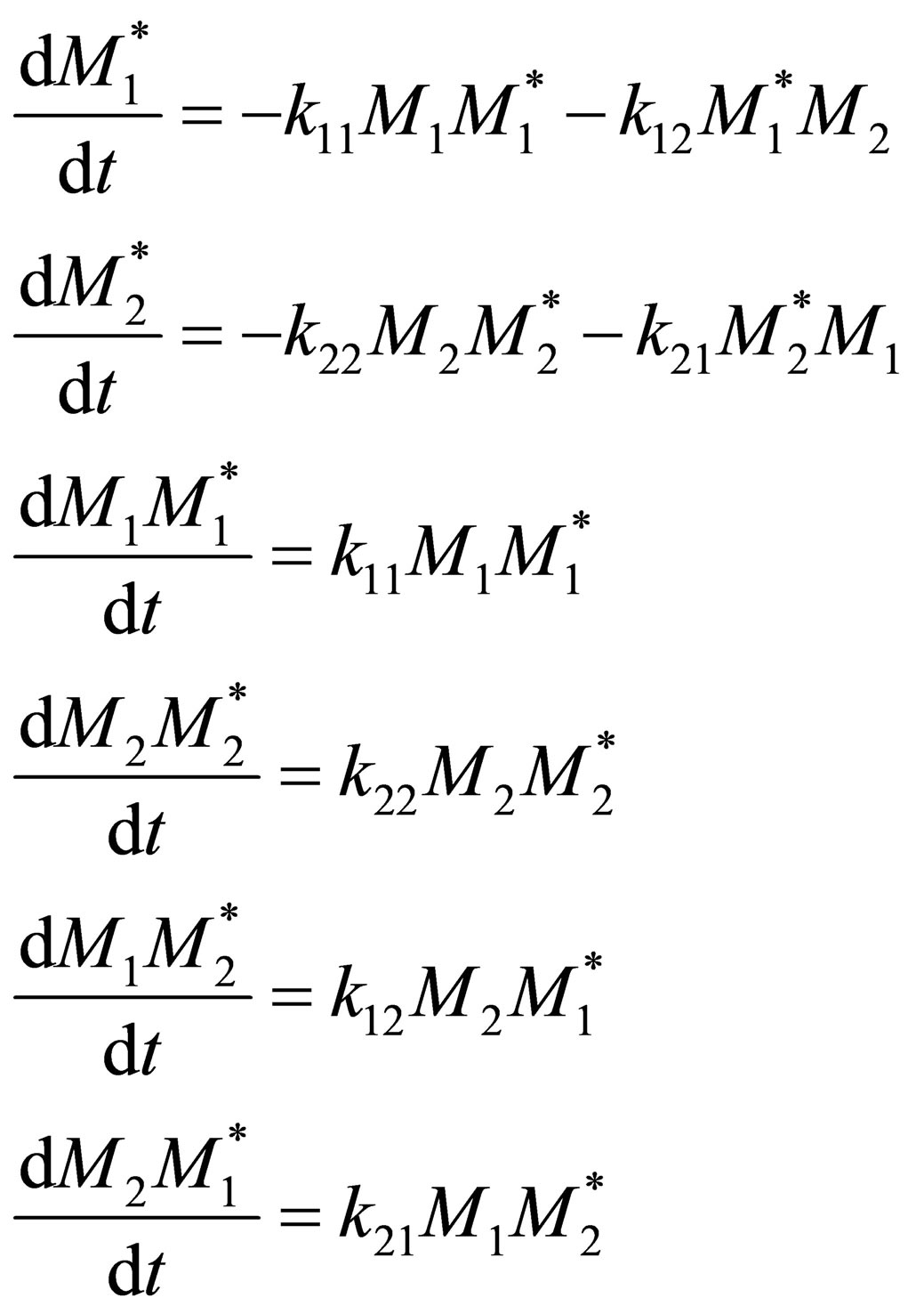 (5)
(5)
By QSSA
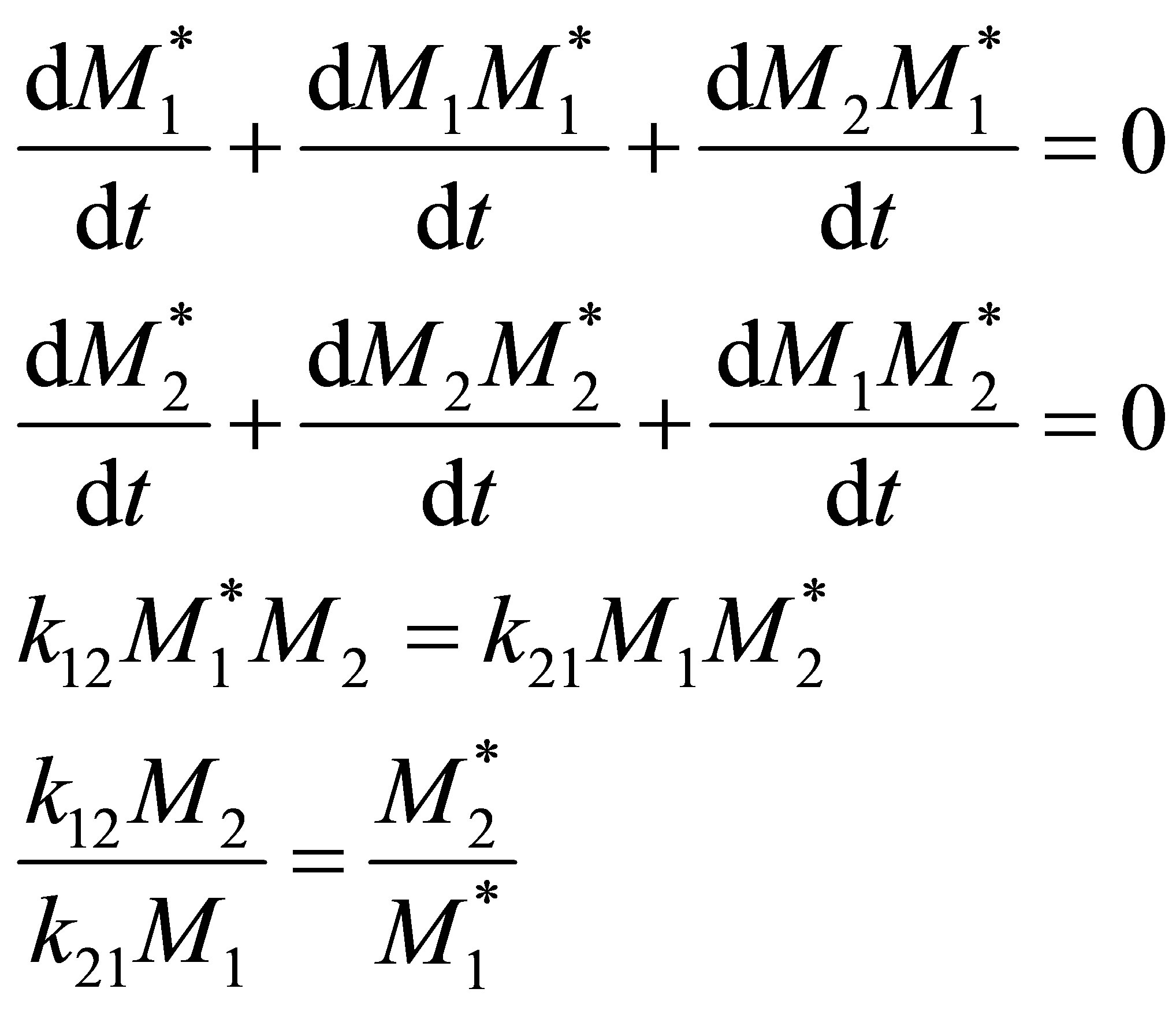 (6)
(6)
The reactivity ratios are defined as follows:
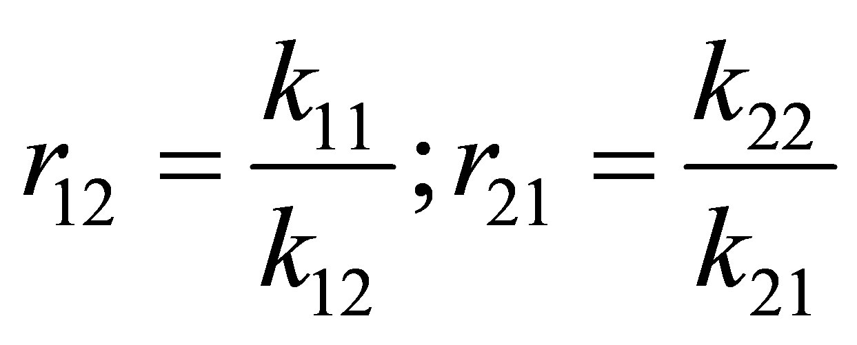 (7)
(7)
Combining Equation (7) and Equation (4);
 (8)
(8)
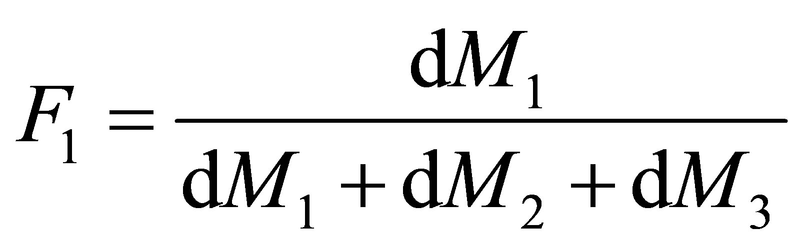
Equation (8) is called the copolymerization composition equation. In a CSTR the effluent concentration and the reactor concentration are the same. The reactor concentration of monomers 1 and 2 are [M1] and [M2] respectively. The polymer composition of monomer 1 repeat unit in the polymer, F1 can be seen to be;
 (9)
(9)
The rate at which the monomer repeat unit 1 enters the copolymer compared with the rates at which all the monomer repeat units enter the backbone of the polymer is given by Equation (9). Equations (8) and (9) can be combined and written as follows:
 (10)
(10)
The concentration of the monomers 1 in the CSTR can be defined as f1:
 (11)
(11)
Or,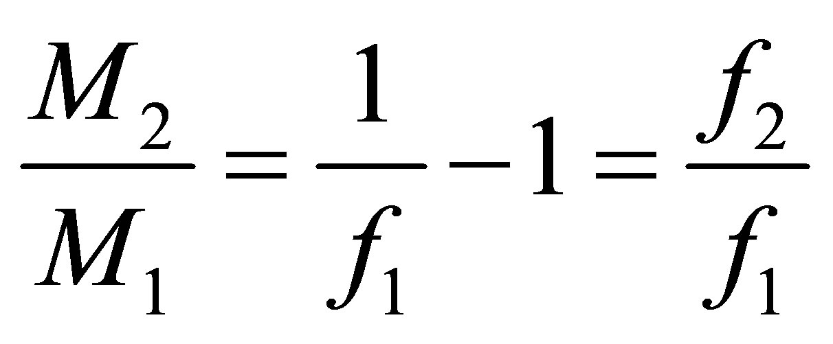 (12)
(12)
An Equation for F1 in terms of f1 can be obtained by combining Equations (10)-(12) as follows:
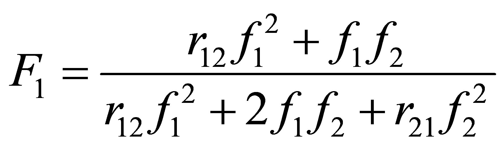 (13)
(13)
The copolymer composition as mole fraction of monomer repeat unit 1 in the polymer as a function of reactor monomer concentrations in CSTR as represented in Equation (1) was developed by Odian [3]. Equation (30) is plotted for different values of reactivity ratios in Figure 2.
It can be seen from Figure 2 that when one of the two reactivity ratios, r12 = r21 = 0 the copolymer is expected to assume the alternating microstructure as shown in introduction section. When one of the reactivity ratios are much greater than 1 block architecture may be expected. The copolymerization is said to be ideal when the product of the two reactivity ratios r12r21 = 1. Here the monomer composition and polymer composition are equal to each other. The copolymer is said to be formed at the azeotropic composition when the monomer and polymer composition are equal to each other.
The copolymer composition vs the monomer concentration in a CSTR for SAN, styrene acrylonitrile and AMS-AN, alphamethyl styrene-acrylonitrile copolymers are shown in Figure 3 The copolymer composition equation changes for AMS-AN copolymers is due to the lack of AMS-AMS propagation reactions. The azeotropic compositions for SAN, AMS-AN copolymers with and without the ceiling temperature effects are shown in Figure 2. It can be seen that the copolymer composition dependence on the monomer composition is sensitive to the reactivity ratios. Even without the ceiling temperature effect the polymer composition for AMS-AN copolymers only changes marginally for a large range of monomer AN compositions. With the ceiling temperature effect it can be seen that the sequence formation of AN-AN dyads, triads, tetrads etc are pronounces in AMS-AN copolymers. More is discussed separately on this topic under sequence distribution of copolymers.
In a PFR, plug flow reactor, the polymer composition can be found by integration of the incremental addition to the polymer across the length of the reactor. During the progression of the monomers in a PFR the composition varies with conversion as follows:
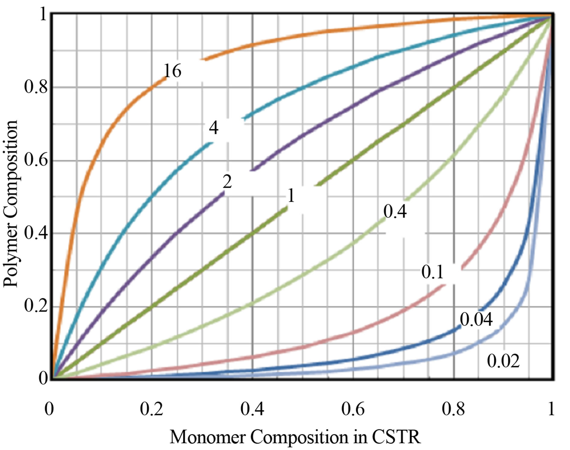
Figure 2. Copolymer composition vs comonomer composition for different reactivity ratios.
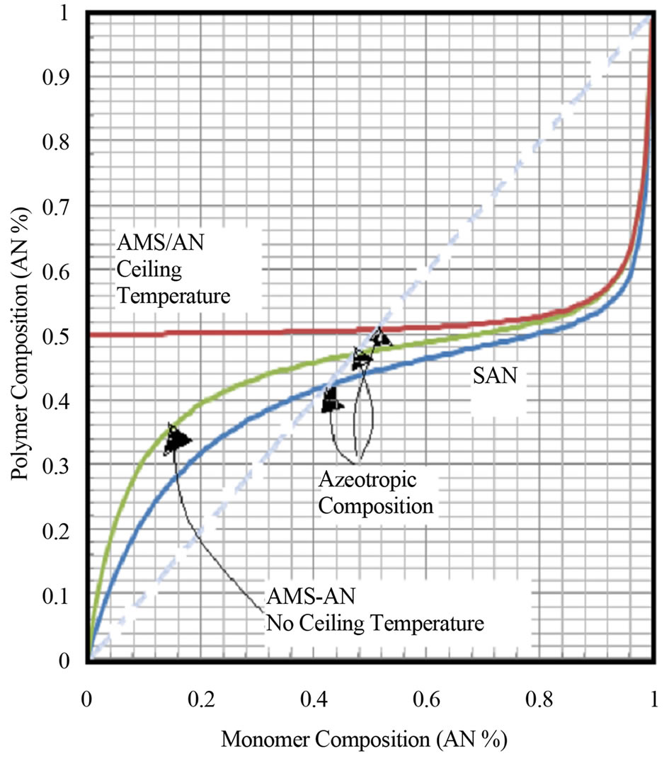
Figure 3. Copolymer composition as a function of monomer composition for SAN and AMS-AN copolymers.
 (14)
(14)
4. Composition of Random Terpolymers
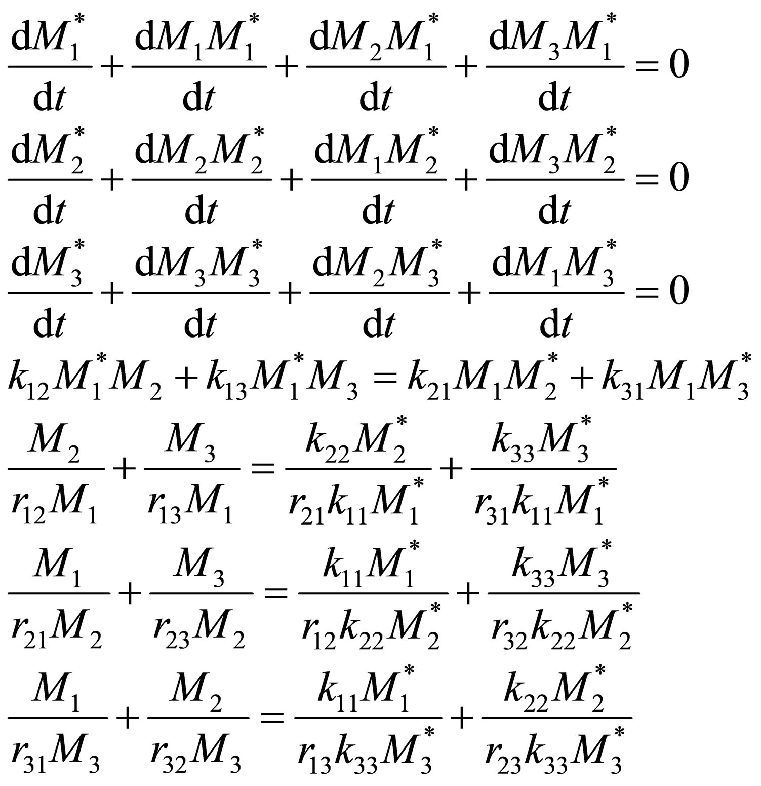
Synthesis of terpolymers has increased in commercial significance over the past few decades. Here the terpolymerization composition equation is derived. Consider three monomer repeat units entering a polymer backbone chain in a CSTR. There are 9 propagation reactions in the case of terpolymerization;
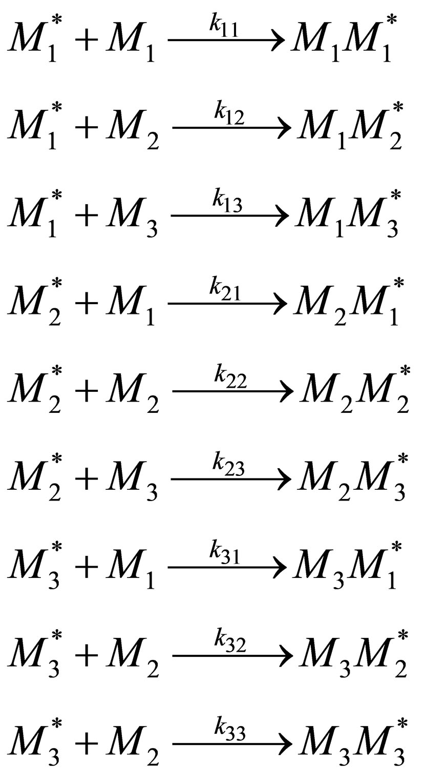 (15)
(15)
The rate of irreversible reactions can be written as follows:
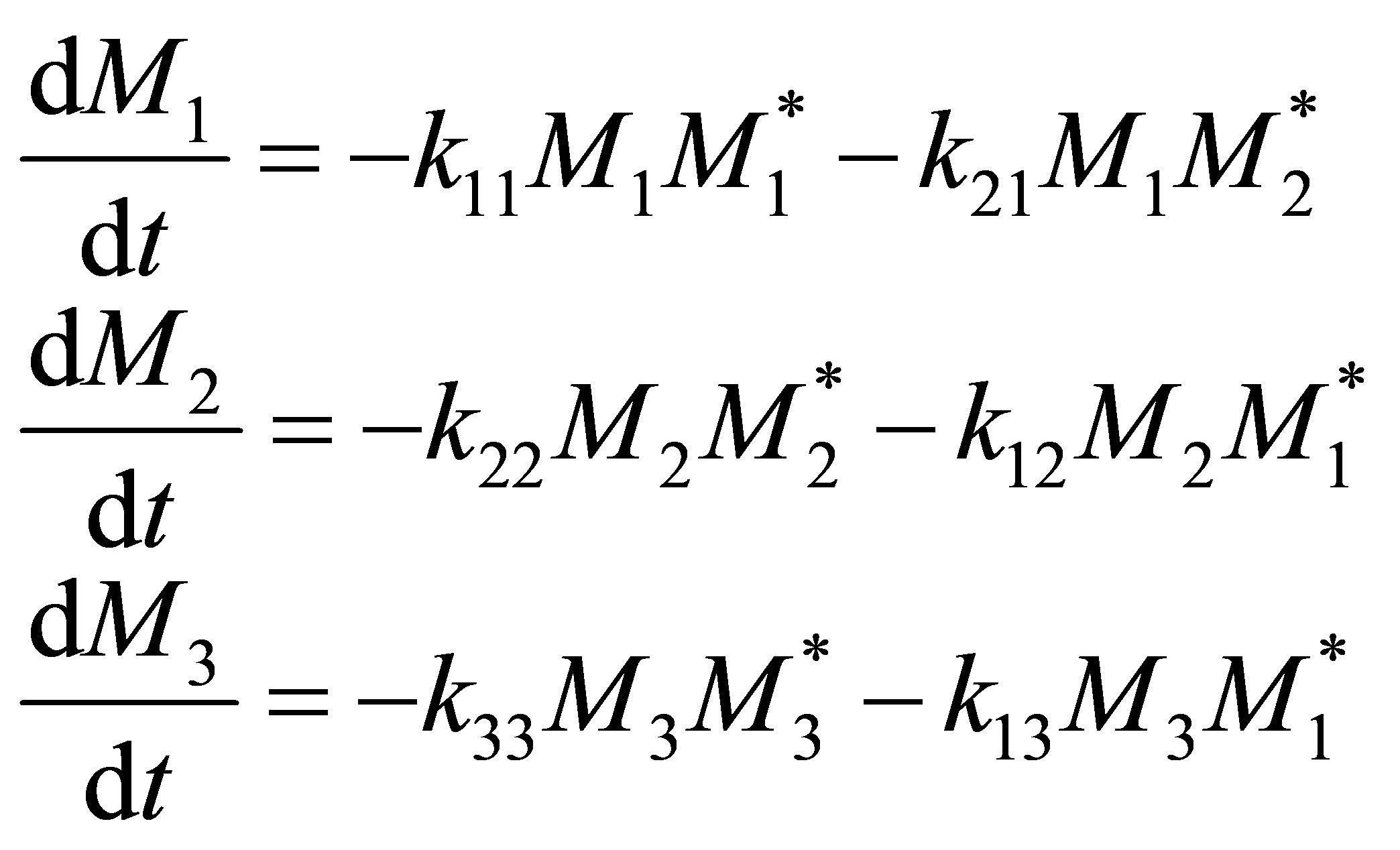 (16)
(16)
The free radical species formed may be assumed to be highly reactive and can assumed to be consumed as rapidly as formed. This is referred to as the quasi-steady state assumption, QSSA.
Thus,
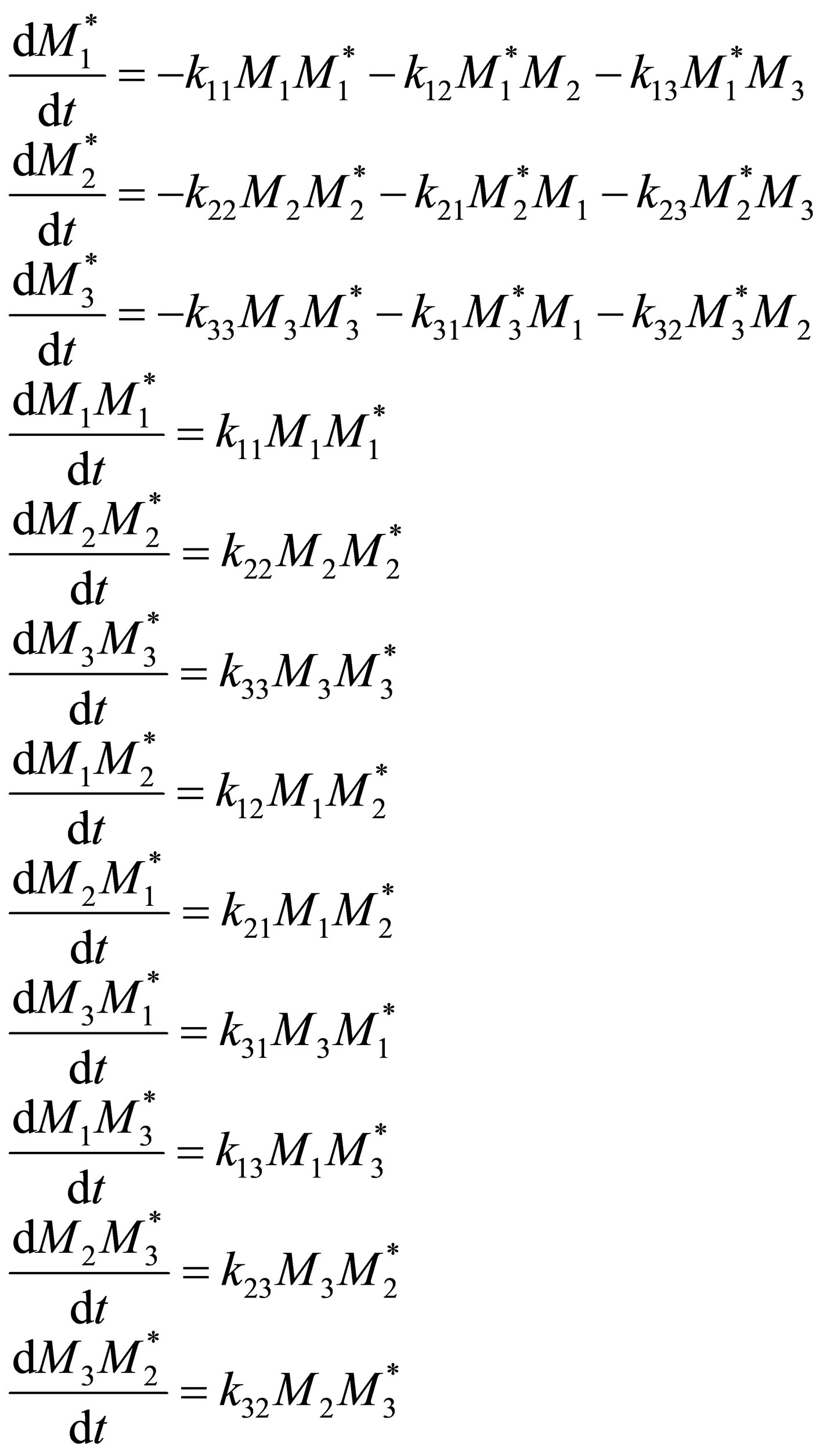 (17)
(17)
By QSSA,
 (18)
(18)
The composition of monomer repeat unit 1 in the terpolymer is given by:
 (19)
(19)
By combination of Equation (16) and the results from QSSA by Equation (18):
 (20)
(20)
In a similar manner reactivity ratios the composition may not be stable. Equation (20) can be re-arranged to provide f1 the composition of the monomers in a CSTR for desired copolymer composition, F1 would be:
 (21)
(21)
5. Sensitivity to Reactivity Ratios
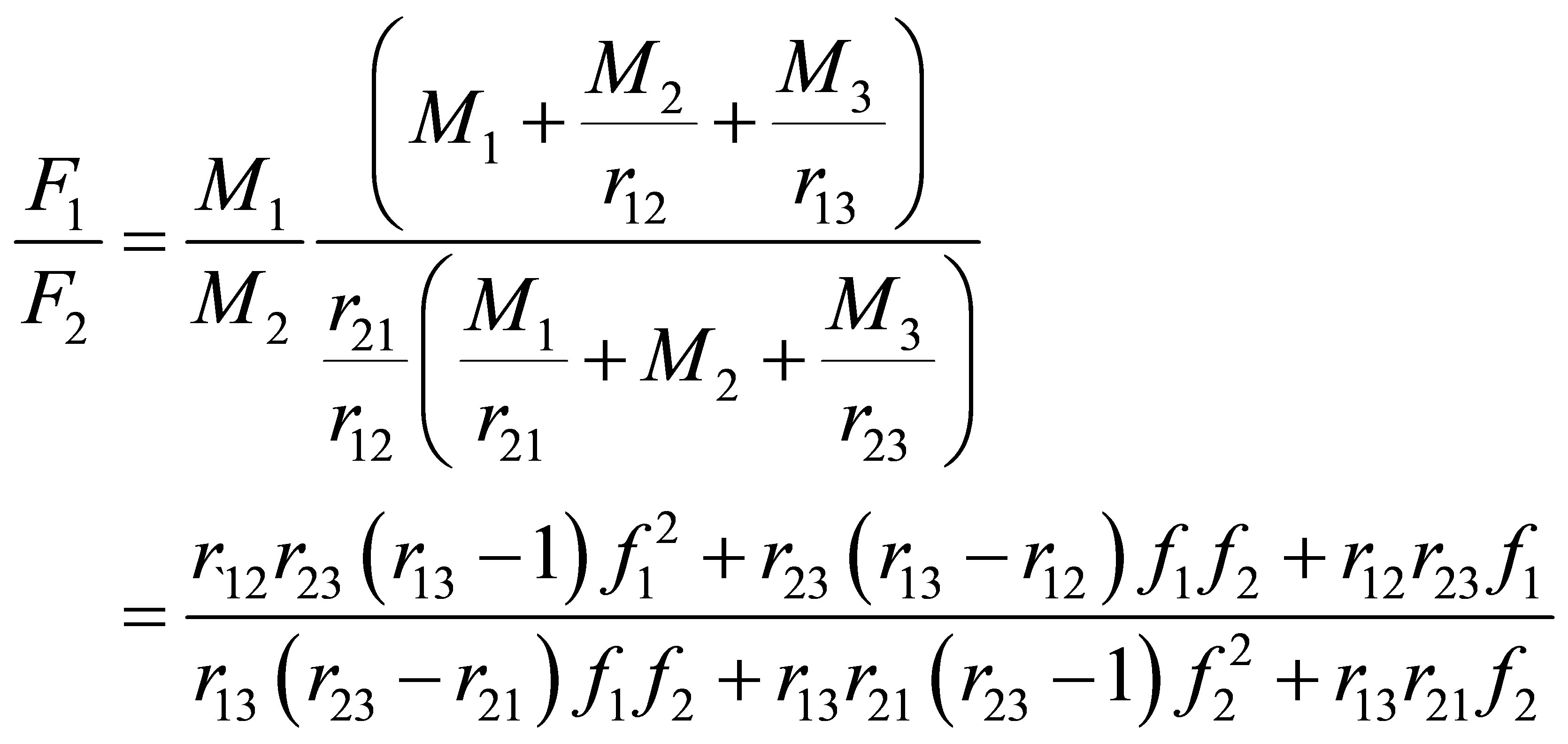
It can be seen that the monomer-polymer composition for terpolymerization in a CSTR will depend on the values of reactivity ratios. Consider the expression derived for the monomer-polymer composition during copolymerization in a CSTR. i.e. Equation (13) rewritten in terms of monomer 1 composition only is:
 (22)
(22)
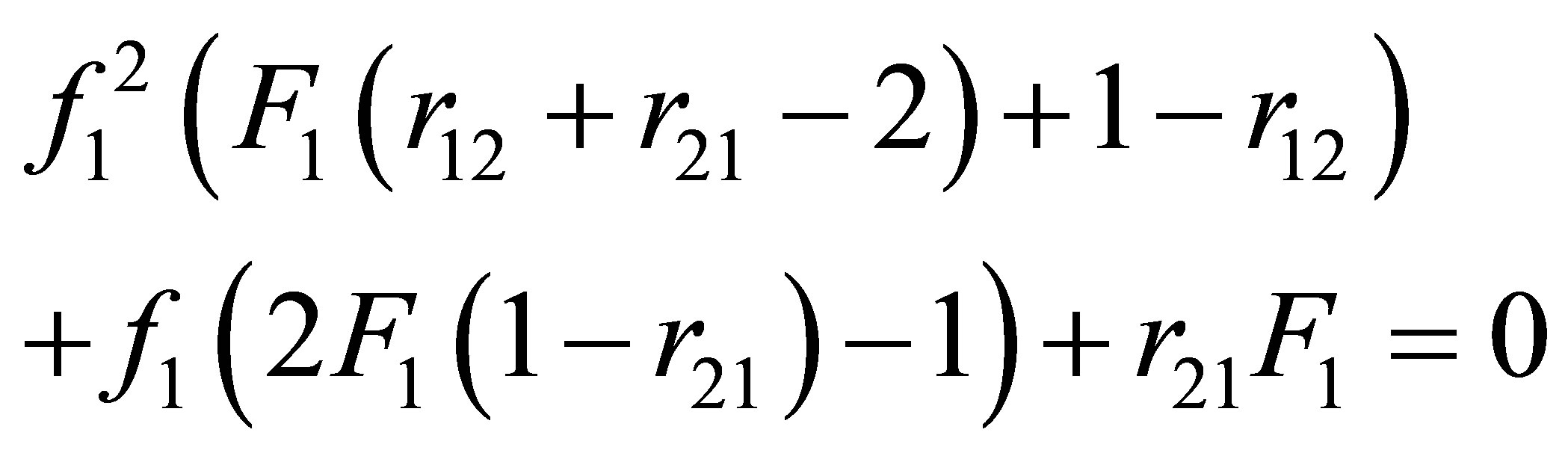
For the particular case when the reactivity ratio value of r12 is 1 or approaches 1, Equation (22) can be seen to become:
 (23)
(23)
Equation (23) can be used to calculate the copolymer composition given the monomer compositions. The inverse problem of finding the monomer composition for a desired polymer composition would need re-arranging Equation (22) and expressing f1 in terms of F1. It appears that the expression would be quadratic in f1. Can this mean that there would be multiple or two roots to a desired polymer composition for some set of reactivity ratios? The monomer and copolymer composition for the system of diethyl fumarate and acrylonitrile is shown in Figure 4.
It can be seen from Figure 4 that for a polymer composition of 30 mole % Diethyl fumarate two monomer compositions of DEF are obtained. This is referred to as multiplicity of compositions. It is not a desirable state to operate the industrial reactors at this composition. Mathematically a quadratic equation can lead to two roots, real or imaginary. This leads to a interesting criteria for copolymer compositional stability. It is conceivable that for some set of reactivity ratios for some polymer compositions two monomer compositions are possible.
The functionality between F1 vs f1 can be seen from Figure 2 and Equation (27) to change from concave to convex curvature as the composition of monomer 1 is increased. The curve inflects. The dependence of polymer composition in the copolymer on the monomer composition in the CSTR depends on the reactivity ratios of the monomers. The reactivity ratios of some commonly used monomers in commercial industrial practice are given in [4].
As an example, the Monomer-Copolymer Composition Curve for the System Methacrylonitrile-Styrene formed in a CSTR is examined. Let the monomer 1 be Methacrylontirle, MAN and monomer 2 be Styrene, STY. It can be seen from that the reactivity ratios r12 and r21 are equal to each other and 0.25. The monomer and copolymer composition curve is shown (Figure 5).
It can be seen from Figure 4 that the copolymer composition curve is S shaped or sigmoidal. Below the azeotropic composition the MAN is favored into the polymer and is more selective. Above the azeotropic composition of 0.5 mole % the Styrene is more selec-
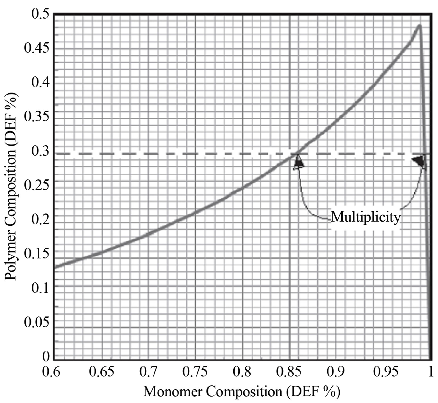
Figure 4. Copolymer composition vs monomer composition in a CSTR for diethyl fumarate and acrylonitrile system.
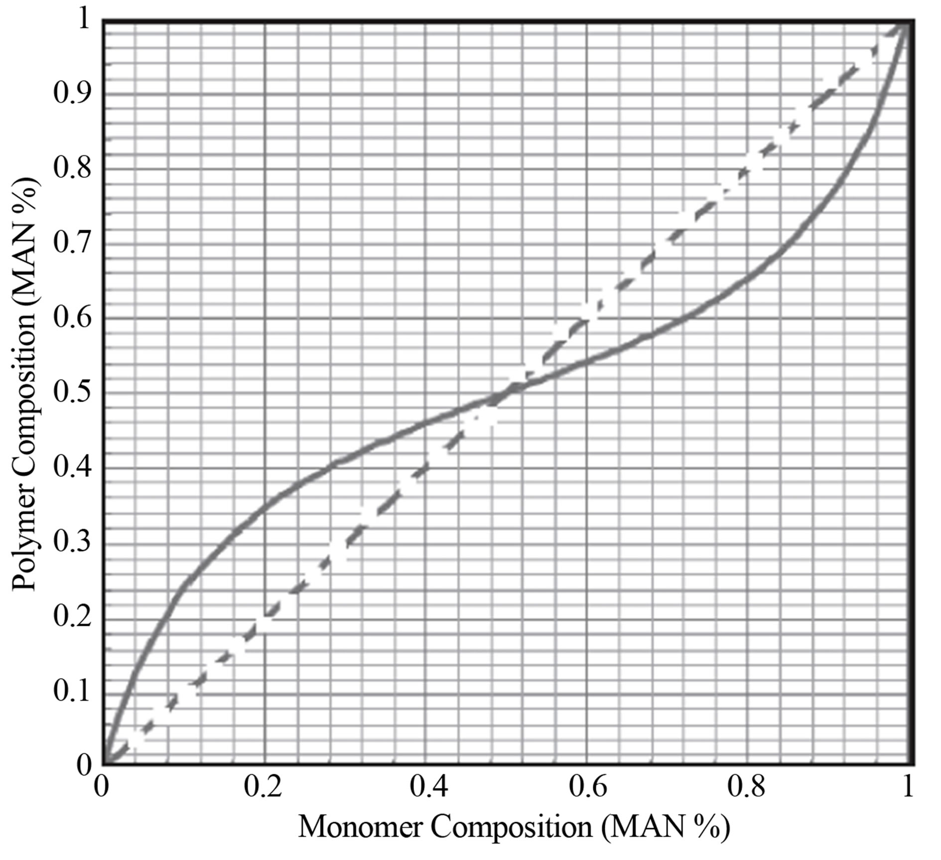
Figure 5. Copolymer composition for MAN-STY vs monomer composition.
tively added into the copolymer chain. As an example the Terpolymer Composition Curves for the Termonomer Systems Acrylonitrile-Styrene-Alphamethyl Styrene by Free Radical Polymerization in a CSTR is examined. Equations (19) and (20) were used to simulate the terpolymer composition curve for different termonomer compositions using a MS Office Excel 2007 Spreadsheet. The reactivity ratios were used from Table 10.1 in Sharma [4]. It can be seen that 5 of the 6 reactivity ratios are less than 1 and one of them r23 is greater than 1. The terpolymer composition of AN at two different compositions of AMS in the monomer phase in a CSTR was plotted in Figure 10.5. The curves were found to be sigmoidal. The AMS composition did not affect the polymer AN composition for monomer compositions less than the 0.45%. Greater than this value AN was found to be more selectively added to the polymer as the AN composition in the monomer phase was increased. Multiplicity in termonomer compositions for a given terpolymer composition can be expected at large values of the reactivity ratios and compositions.
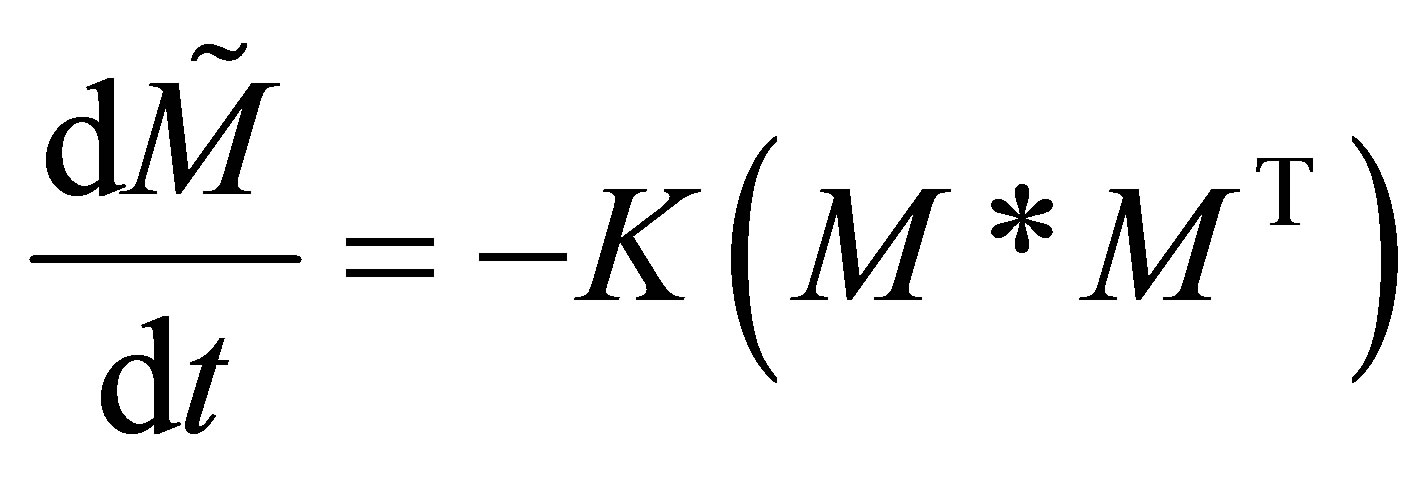
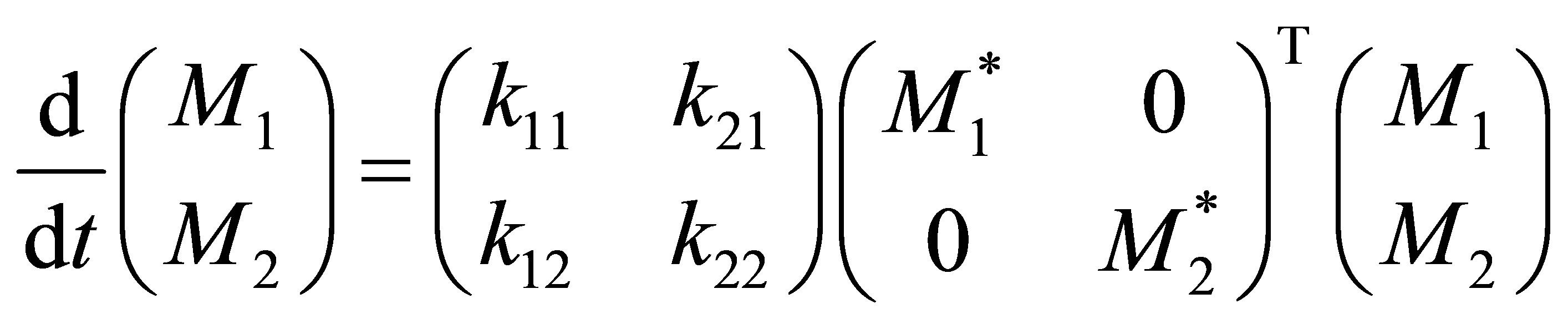
6. Multi-Component Copolymerization— n Monomers
The analysis on copolymerization and terpolymerization resulting in copolymer composition vs monomer composition relations in the prior sections can be generalized to n monomers. Consider n monomer repeat units entering a polymer backbone chain in a CSTR. There are n2 propagation reactions that can be involved in the multicomponent copolymerization. Thus for tetrapolymerization there would be 16 propagation reactions involved. These reactions are listed below:
 (24)
(24)
The rate of irreversible reactions can be written correspondingly for n monomers similar to Equations (5) and (17) written for copolymer and terpolymer.
The free radical species formed may be assumed to be highly reactive and can assumed to be consumed as rapidly as formed.
This is referred to as the QSSA, quasi-steady state assumption.
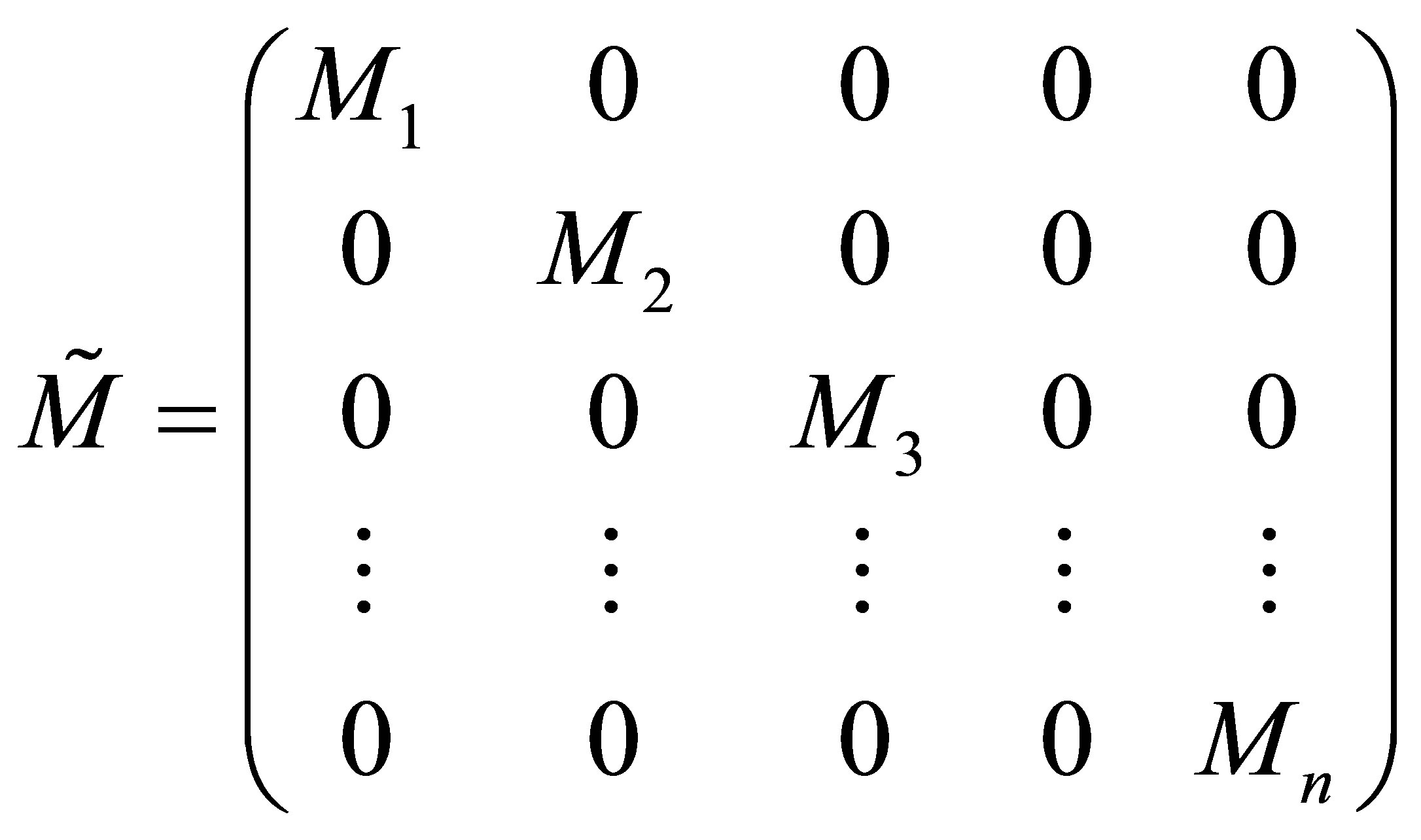
Let the n monomer concentrations be represented by the vector M and n free radical concentrations by represented by vector M* as;
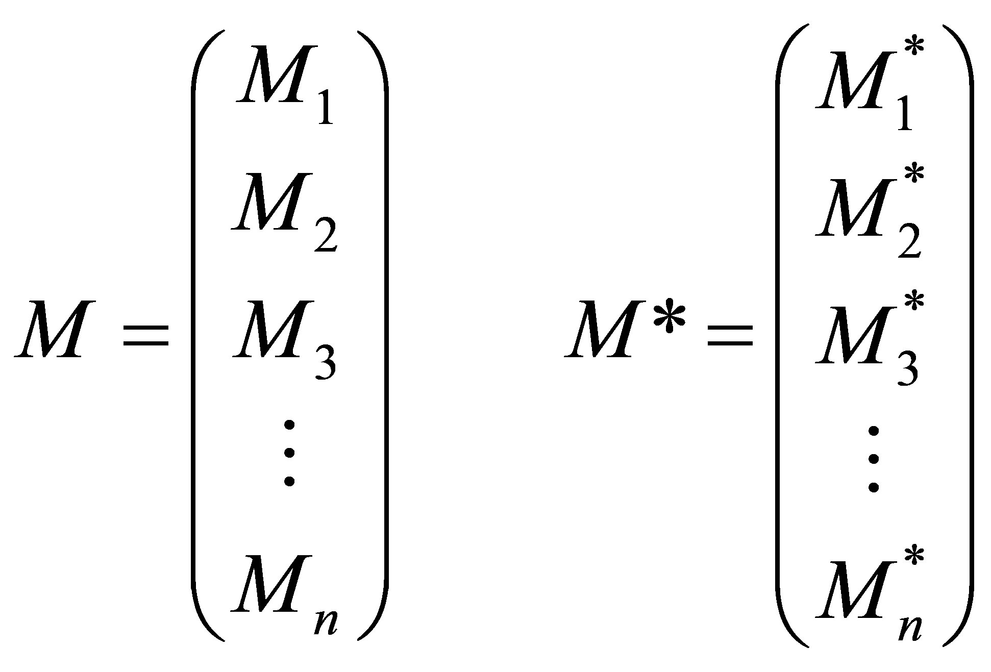 (25)
(25)
The multi-component copolymerization rate constants can be represented by a rate matrix as follows:
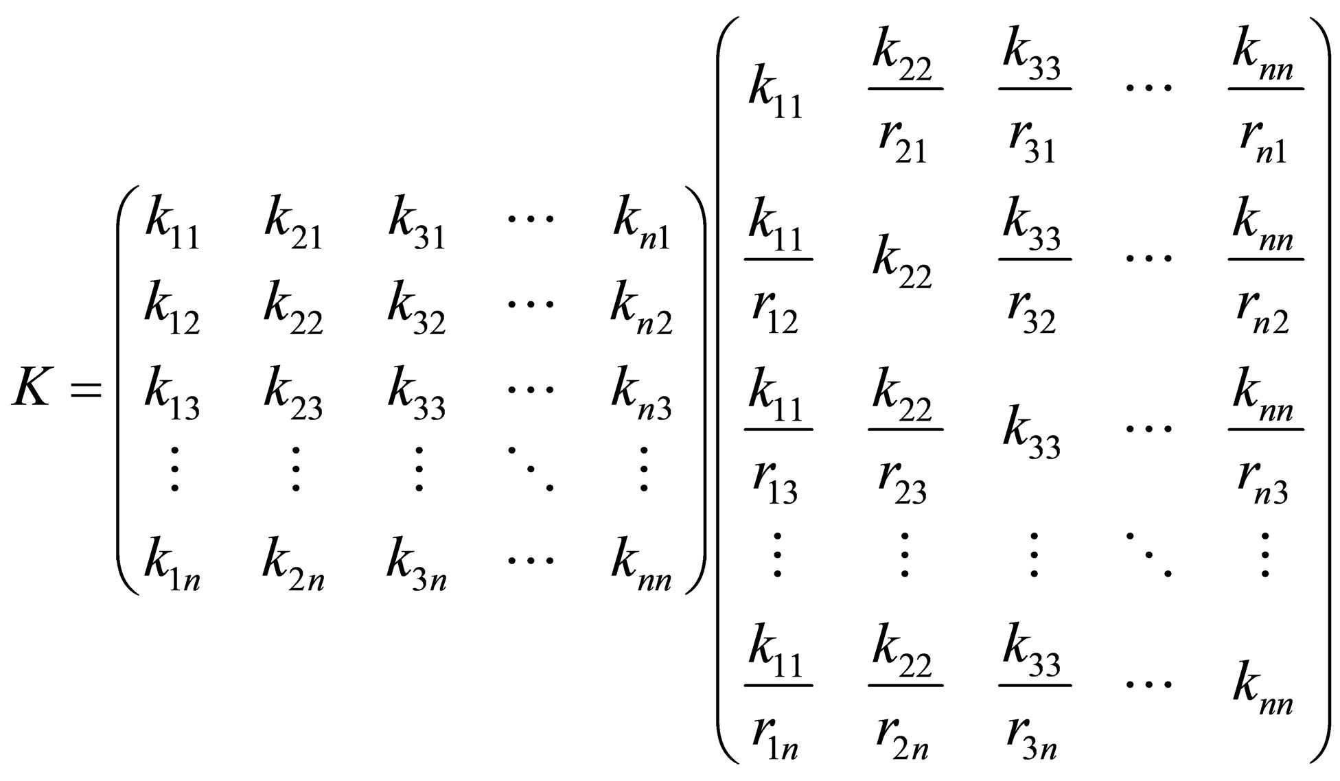 (26)
(26)
The rate matrix for multi-component copolymerization can thus be also be expressed in terms of the homopolymerization propagation rate constants of the n monomers respectively and reactivity ratios as defined in a similar manner to Equation (5). The set of copolymerization rate equationsfor n monomers can be given in the matrix form as follows:
 (27)
(27)
where,
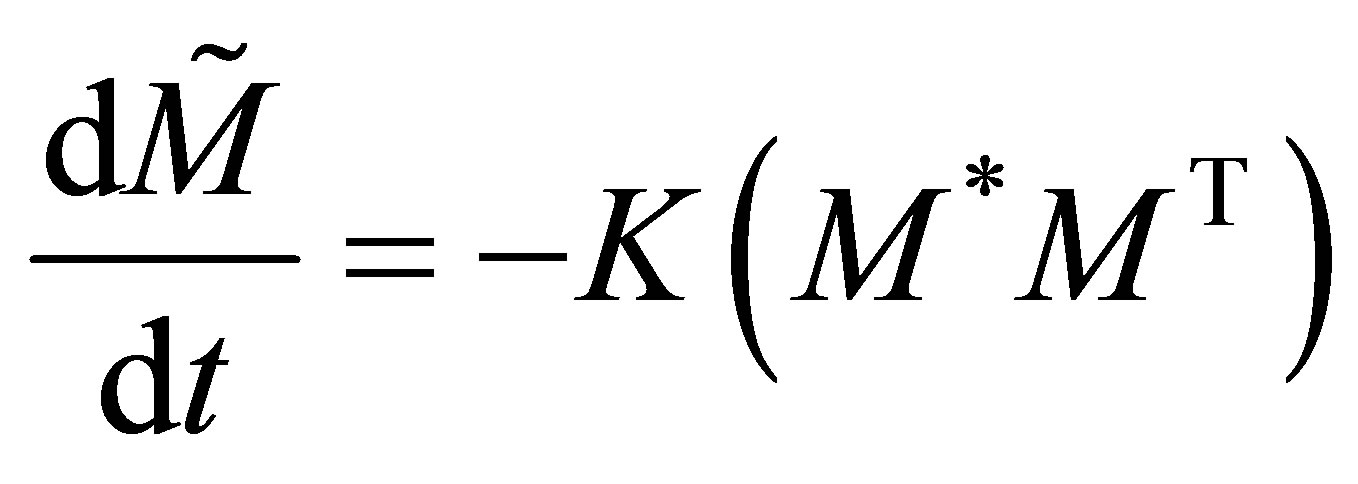
Only the diagonal elements of the resulting matrix from the RHS, right hand side of Equation (27) is of interest. The rate equations that represent the radical generation and consumption during propagation can be given in the matrix form as:
 (28)
(28)
Equations (31) and (33) form a set of autonomous systems. For certain values of the rate propagation matrix using Eigenvectors and stability analysis it can be shown that periodic solutions may result. The initial conditions of the monomers can be represented by:
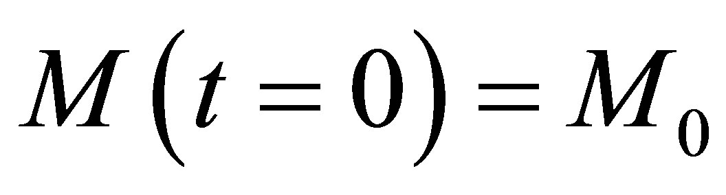 (29)
(29)
By the QSSA, quasi-steady state assumption, i.e., the radical species are highly reactive, Equation (28) can be set to zero. Or
 (30)
(30)
For a given set of reactivity ratios, homopolymer propagation constants and initial condition of multicomponent comonomers, M* can be solved for by using Equation (30) and then substituted in Equation (28). Then the monomer concentrations with time as well as the polymer composition can be calculated from Equation (27). Equation (28) can be solved for by the method of Eigenvectors [5]. It can be seen that non-trivial equations to the set of ordinary differential equations with constant coefficients represented by Equation (28) exist only for certain specific values of l called Eigenvalues. These are the solutions to:
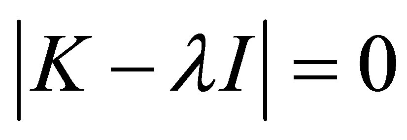 (31)
(31)
Equation (31) can be expanded into a polynomial degree n in l:
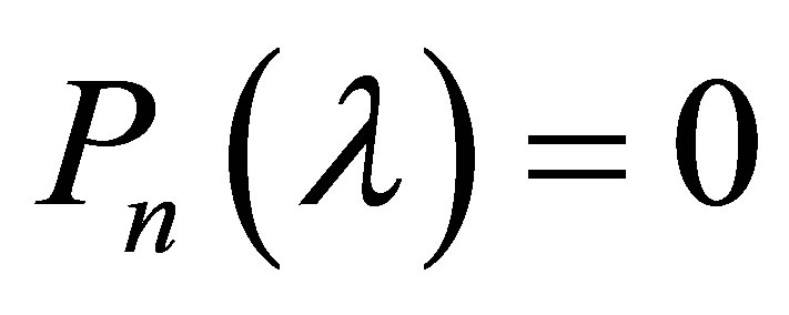 (32)
(32)
In order to obtain numerical values for Eigenvalues, the expansion of Equation (32) is considered obtained by Laplace development of the determinant:
 (33)
(33)
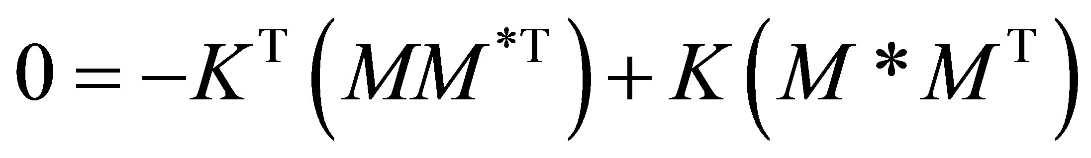
where, 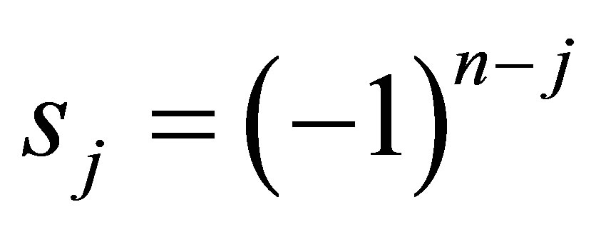 sum of all principal minors of order j of K where
 .
.
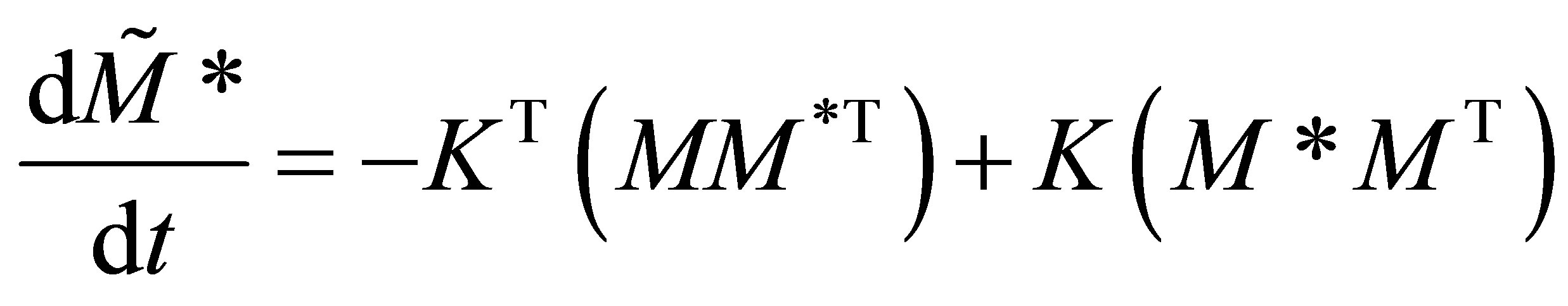
The copolymer composition can be obtained using the trace of the matrix defined in Equation (31). Trace is a sum of all the diagonal elements of a matrix. Thus;
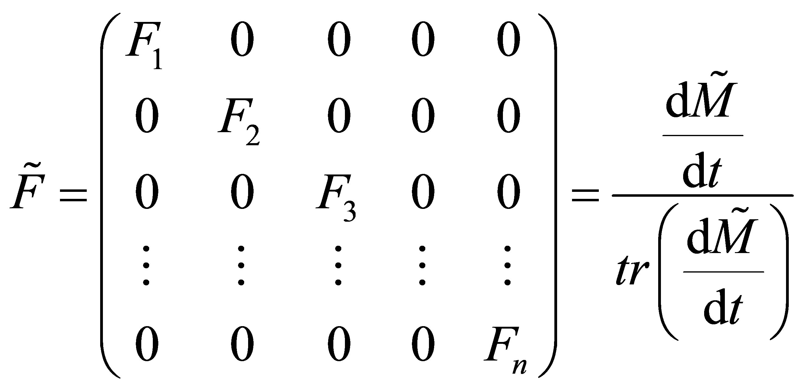 (34)
(34)
The corresponding monomer compositions in the CSTR for n comonomers entering the copolymer backbone chain can be written as follows;
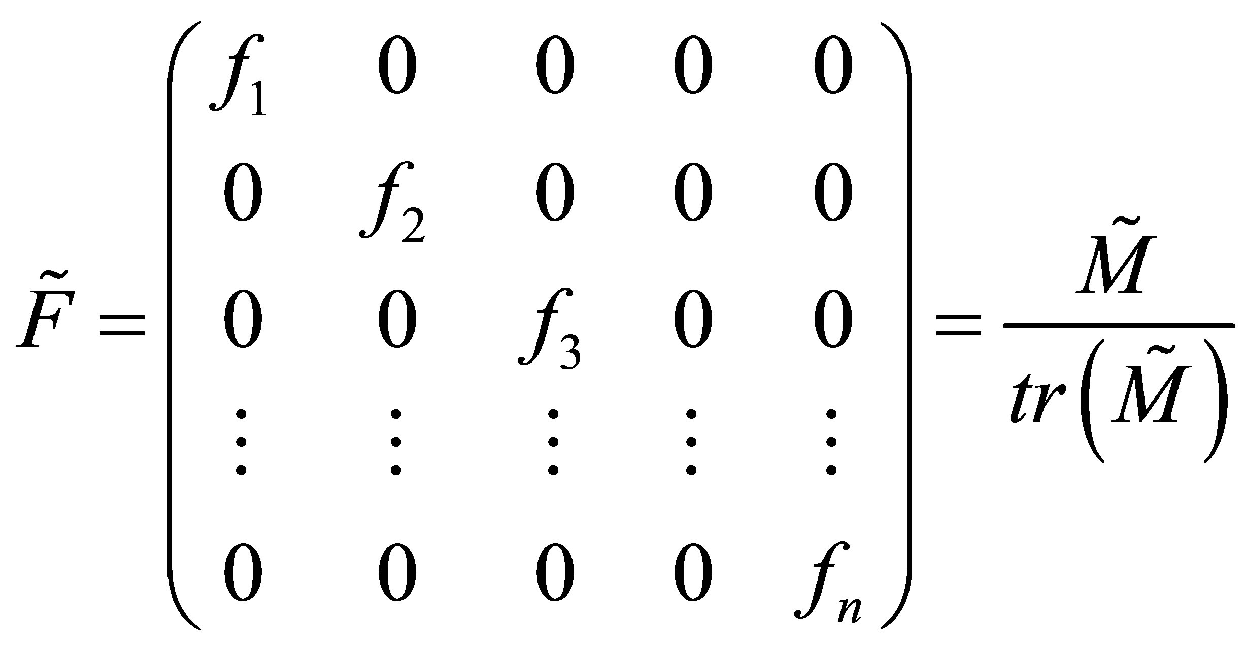 (35)
(35)
Equation (35) can be differentiated with respect to time and combined with Equation (34) to obtain the relation between the multi-component copolymer composition and CSTR monomer compositions. It can be realized that trace of a square matrix is a scalar quantity. Equation (31) is in terms of MT and diagonal matrix . During copolymerization from the QSSA as given by Equation (4) it can be seen that:
 (36)
(36)
This is because the bond  and
and  are formed at the same rate. The order of addition of the radical does not matter. Equation (36) can also be shown to be case by evaluation of Equation (37)
By QSSA it can be seen that Equation (37) ought to be set to 0. Differentiating the resulting equation with respect to time:
 (37)
(37)
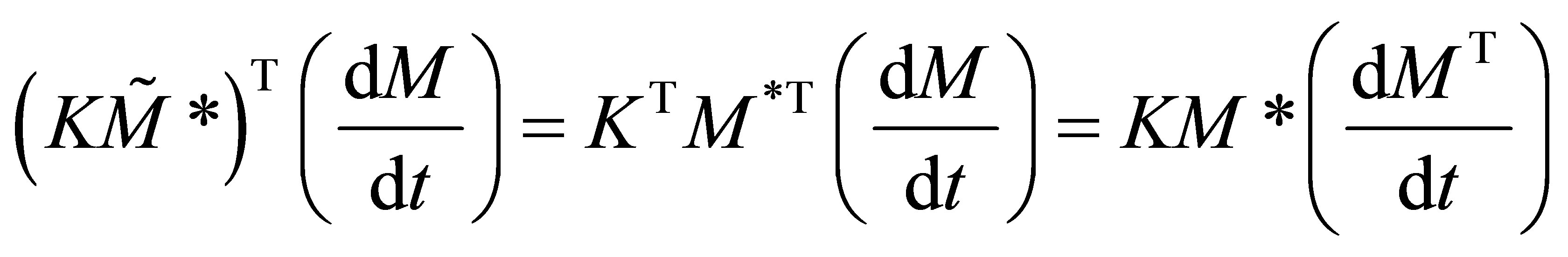 (38)
(38)
It can be seen from Equation (38) that;
 (39)
(39)
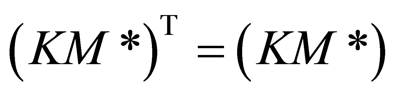
Equation (36) would fall out from Equation (39) when the order of the matrix is 2. Subsituting Equation (36) in the set of copolymerization rate equations the rate matrix can be rewritten as:
 (40)
(40)
 (41)
(41)
Equation (40) is a reasonable assumption for multicomponent copolymerization for the general case of n monomers as well. This implies that the rate of copolymerization propagation of  equals the formation of
  radical. When this is applied to all possible pairs of monomers in n comonomers the QSSA holds as the net production of radicals equals the consumption during the copolymerization propagation itself. Nothing about the termination reactions are brought forward into this analysis. Thus for n comonomers Equation (42) can be written.
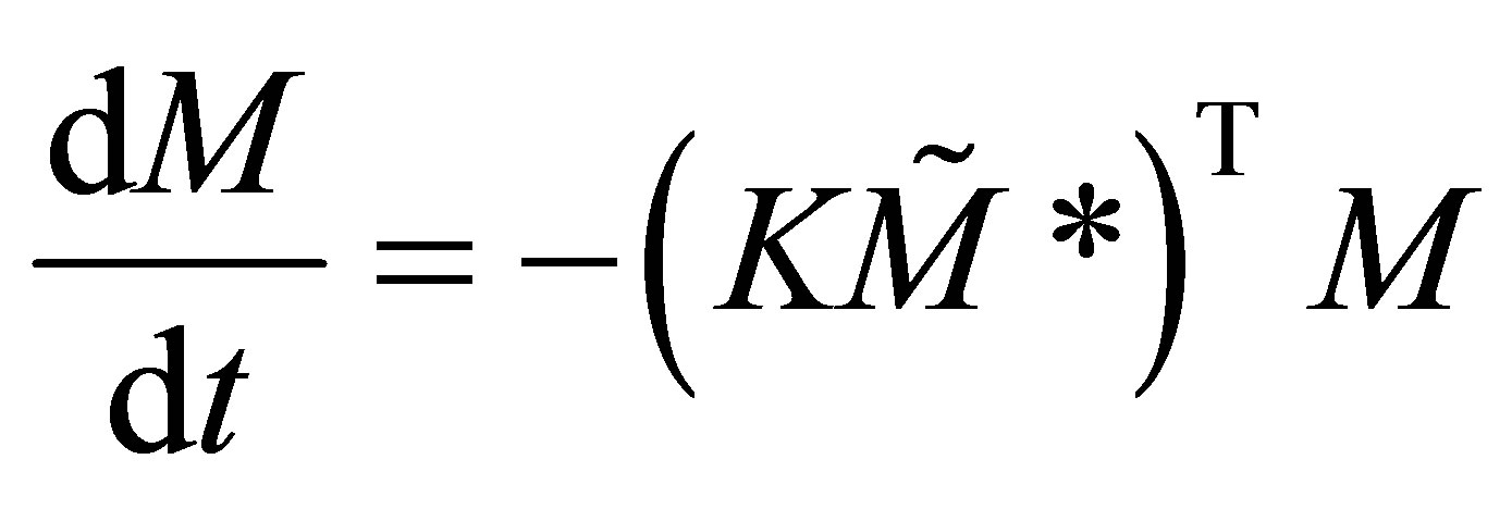
The solution to Equation (42) can be obtained by the method of Eigenvectors. Assume that the solution to Equation (42) has the form;
 (43)
(43)
where Z is the unknown vector of constants and are the Eigenvalues. Substituting Equation (43) in Equation (41):
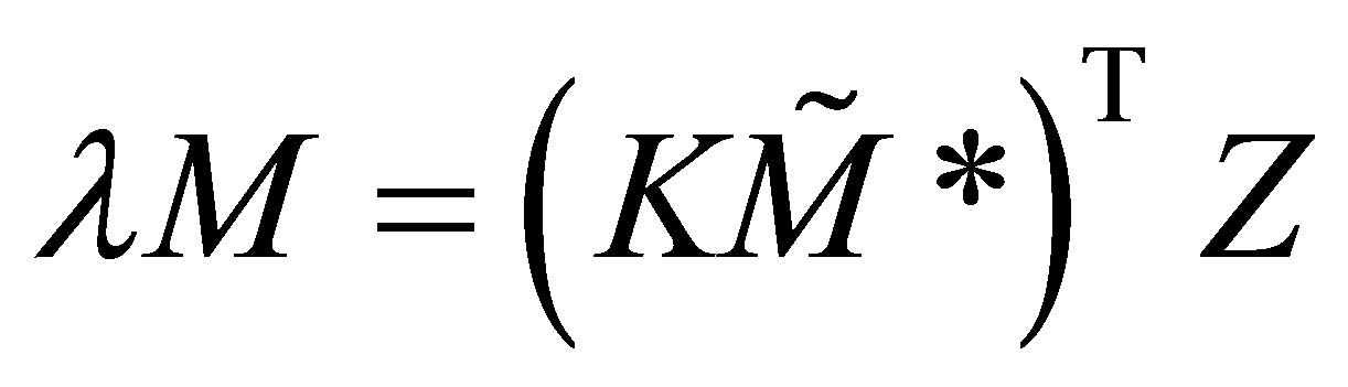 (44)
(44)
Equation (44) requires that elt ≠ 0. It is assumed that the form of the solution to the set of ordinary differential equations with constant coefficients is as given in Equation (43). This requires that Z ≠ 0. It can be seen from Equation (46) that is an Eigenvalue of the rate matrix modified with the free radical concentrations. The free radical concentrations can be obtained from Equation (34). The modified rate matrix transposed, is a square matrix of n × n. Therefore n Eigenvalues can be expected. The Eigenvalues must obey;
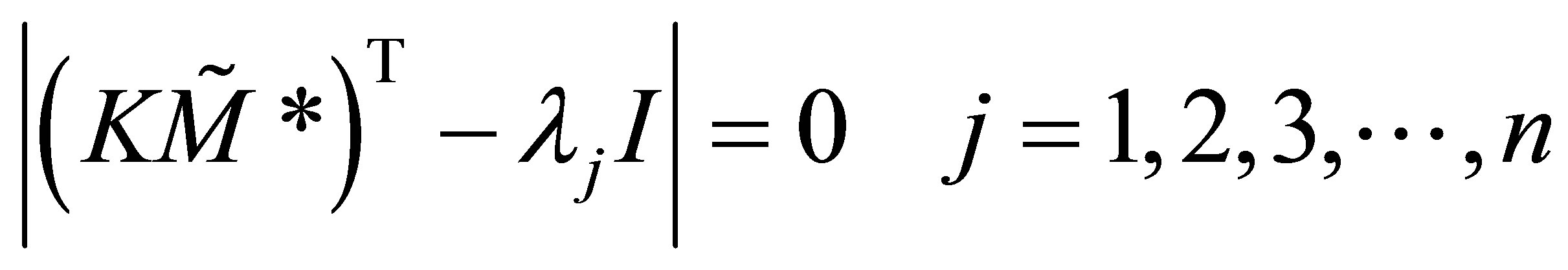 (45)
(45)
Corresponding to each Eigenvalue exists an Eigenvector Zj. Thre are n solutions of the form of Equation
(45). The general solution of the homogeneous equation Equation (45) is given by a linear combination of these solutions as:
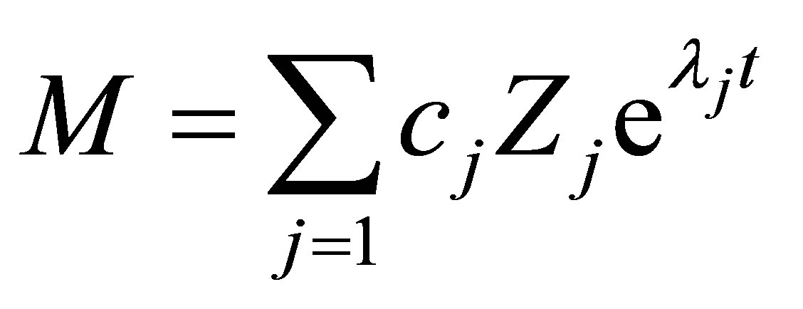 (46)
(46)
where cj are integration constants that can be solved for from the initial condition given by Equation (29). When the Eigenvalues when solved for from the polynomial equation given by Equation (33) becomes complex the solution to the monomer concentration with time becomes subcritical damped oscillatory (Sharma [6-23]).
7. Transient Conversion in Continuous Stirred Tank Reactor, CSTR
7.1. Thermal Initiation Polymerization
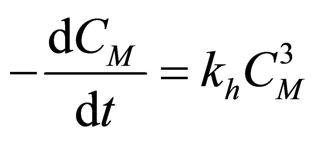
Example 1: Monomers such as styrene can be polymerized using thermal initiation. At higher temperatures the styryl radical forms. This initiation is called thermal initiation. The rate of the initiation reaction is of the third order. There are reports in the literature to the formation of a Dields Alder mechanism. These reactions are important in the manufacture of polystyrene, HIPS, high impact polystyrene, SAN, styrene acrylonitrile copolymer, ABS, acrylonitrile, butadiene and styrene engineering thermoplastic etc. Allow these reactions to be performed in a CSTR (Figure 6). Assume that the flow is incompressible and the reactor is operated at constant volume. Discuss the transient monomer concentration in the CSTR. Use the dimensionless group Damkohler number, conversion, dimensionless time, if necessary. The free radical reactions of initation, propagation and termination are given as follows:
Thermal Initation
 (51)
(51)
Monomer Propagation
 (52)
(52)
| |
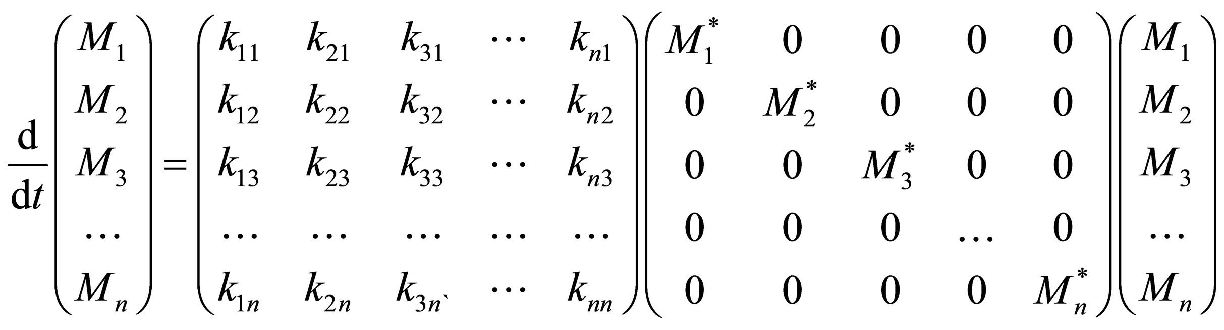
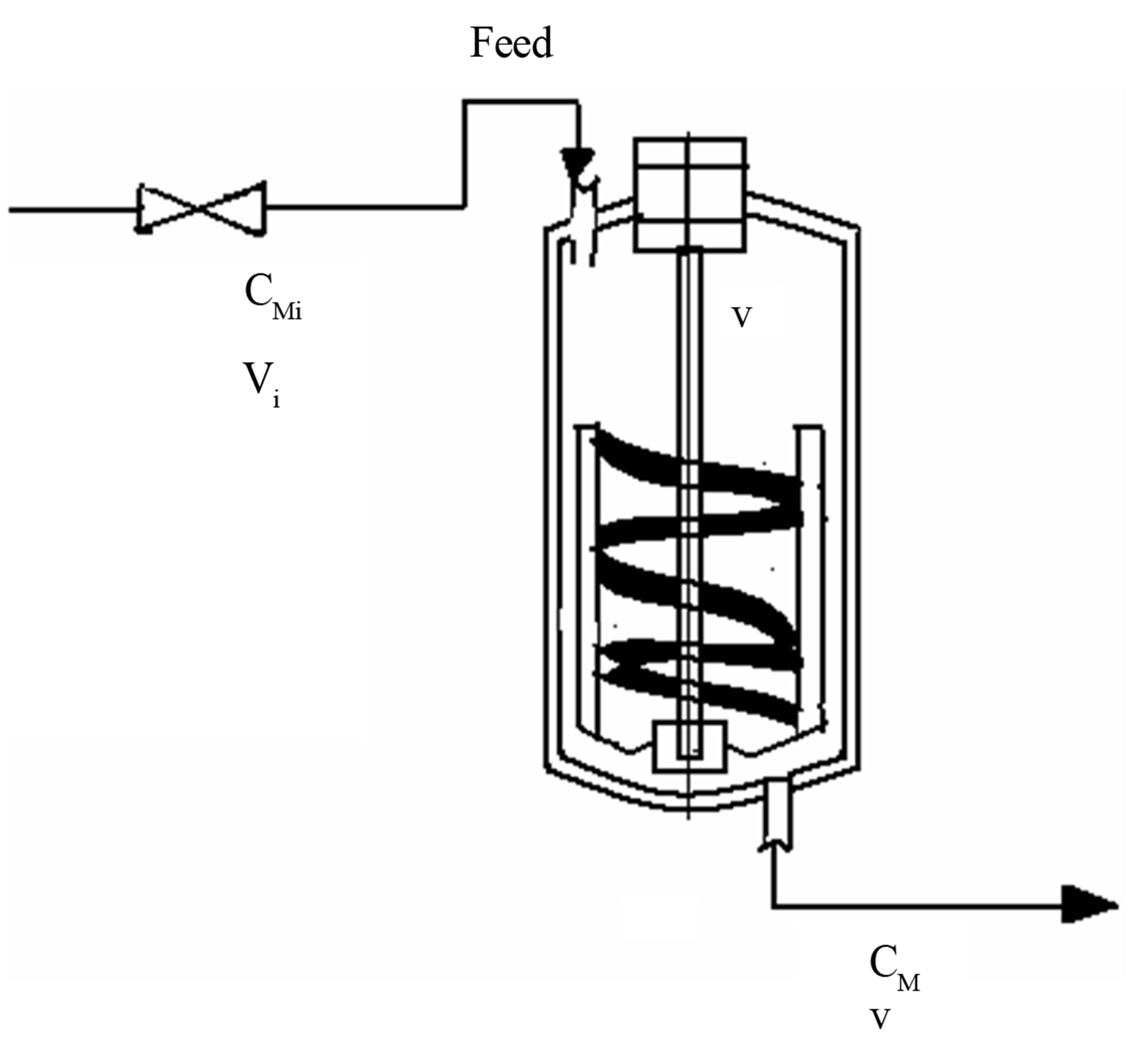
Figure 6. Continuous stirred tank reactor, CSTR operated at constant volume, V.
Monomer Termination
 (53)
(53)
From the assumptions of incompressible flow and constant volume reactor, it can be seen that
 (54)
(54)
Hence, . Note that this is by inference from incompressible flow and not from steady state considerations. Therefore,
 . A component balance on the monomer that is polymerized in the CSTR can be written as follows;
 (55)
(55)
The rate of polymerization (rp) can be arrived at as follows:
Rate of Initiation
 (56)
(56)
Rate of Propagation Assuming that the propagation reactions are fast that the rate coefficient is independent of the length of the radical chain:
 (57)
(57)
Rate of Termination
 (58)
(58)
The “pseudo-steady state” assumption can be used to obtain an expression for the radical concentration during polymerization. The radicals formed during propagation get consumed immediately in the next step. The net rate of production of radicals is zero. Hence the rate of initiation and rate of termination can be added to zero as follows:
 (59)
(59)
The expression for the concentration of the free radicals is:
 (60)
(60)
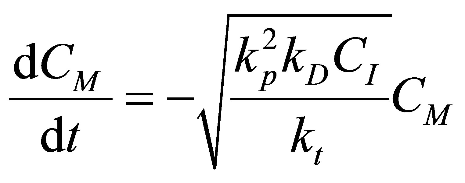
Consequently, the rate of polymerization, (rp) can be seen to be:
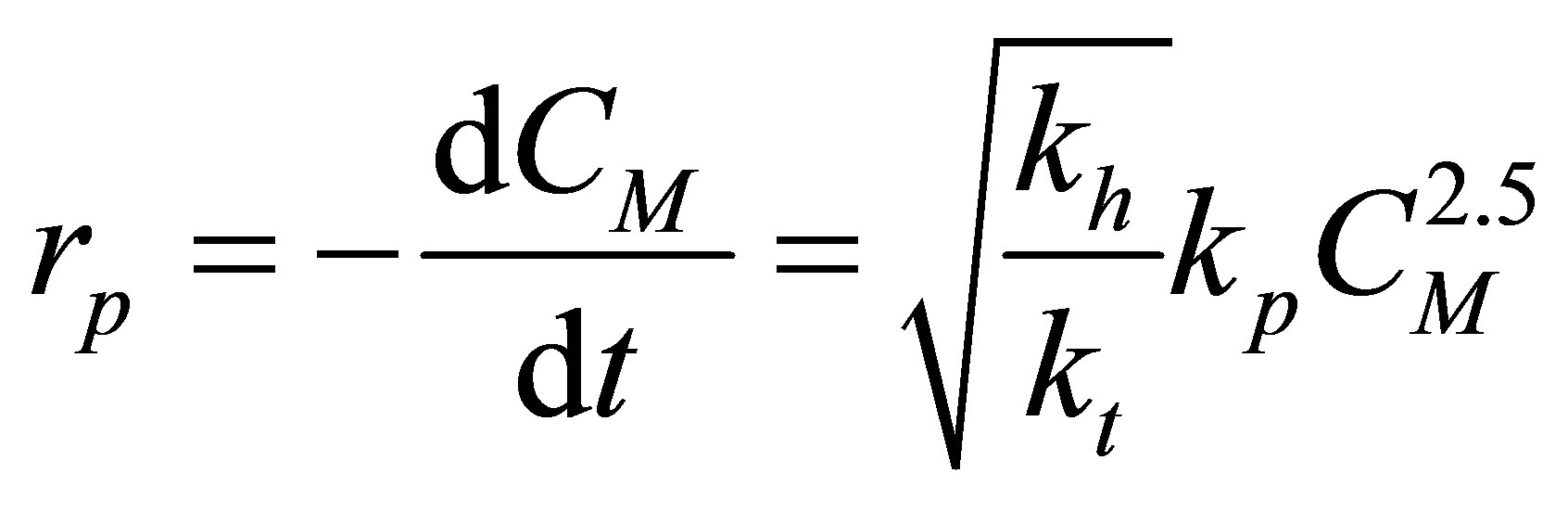 (61)
(61)
The monomer component mass balance equation becomes:
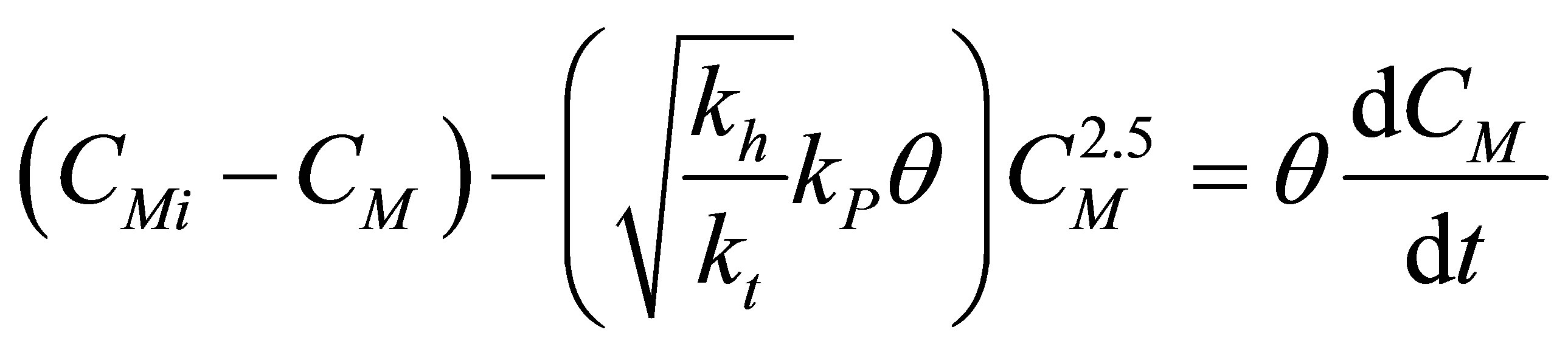 (62)
(62)
Define the dimensionless groups as follows:
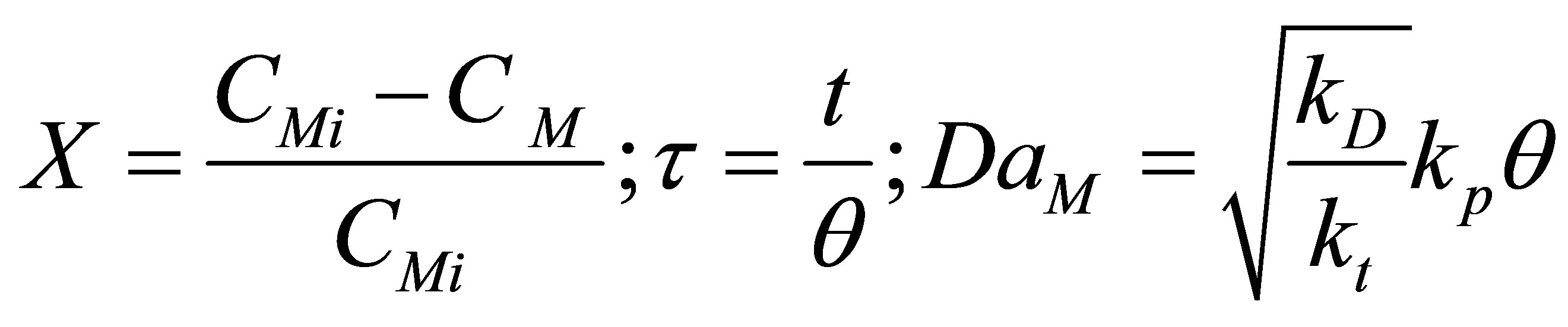
Fractional Conversion, XM
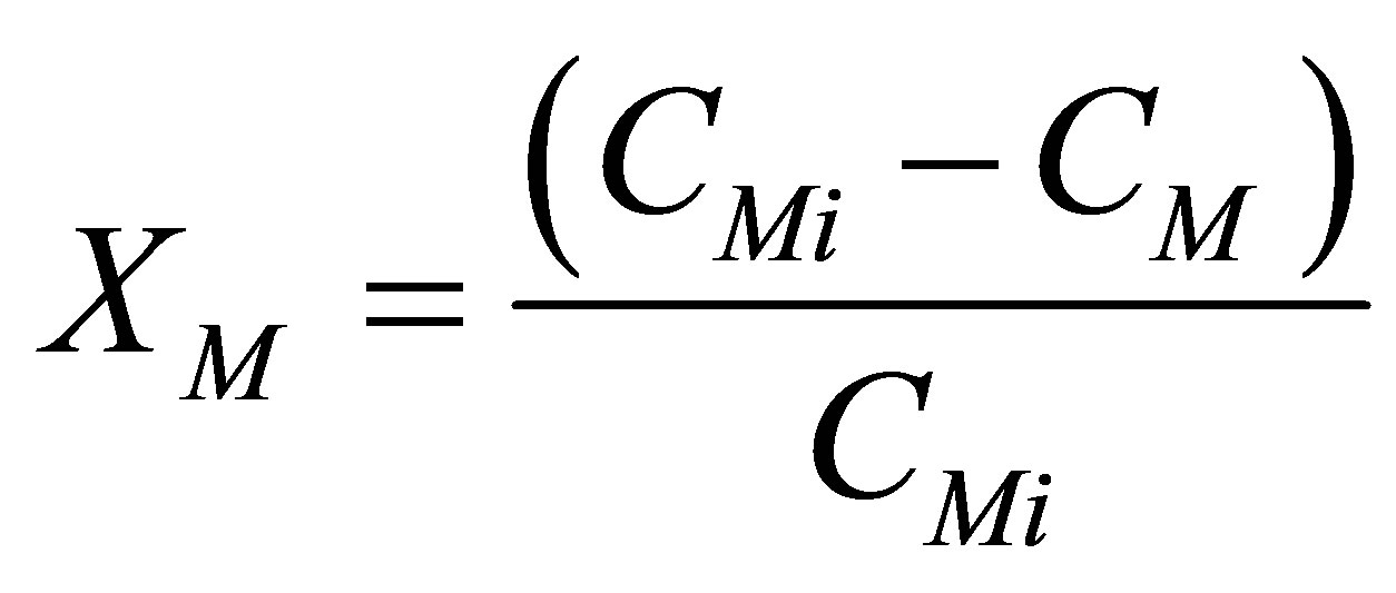 (63)
(63)
Dimensionless time, t
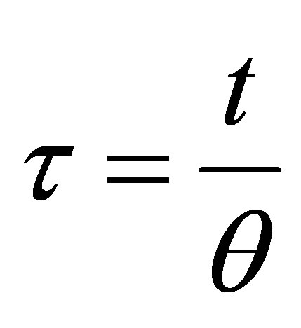 (64)
(64)
Damkohler Number, DaM
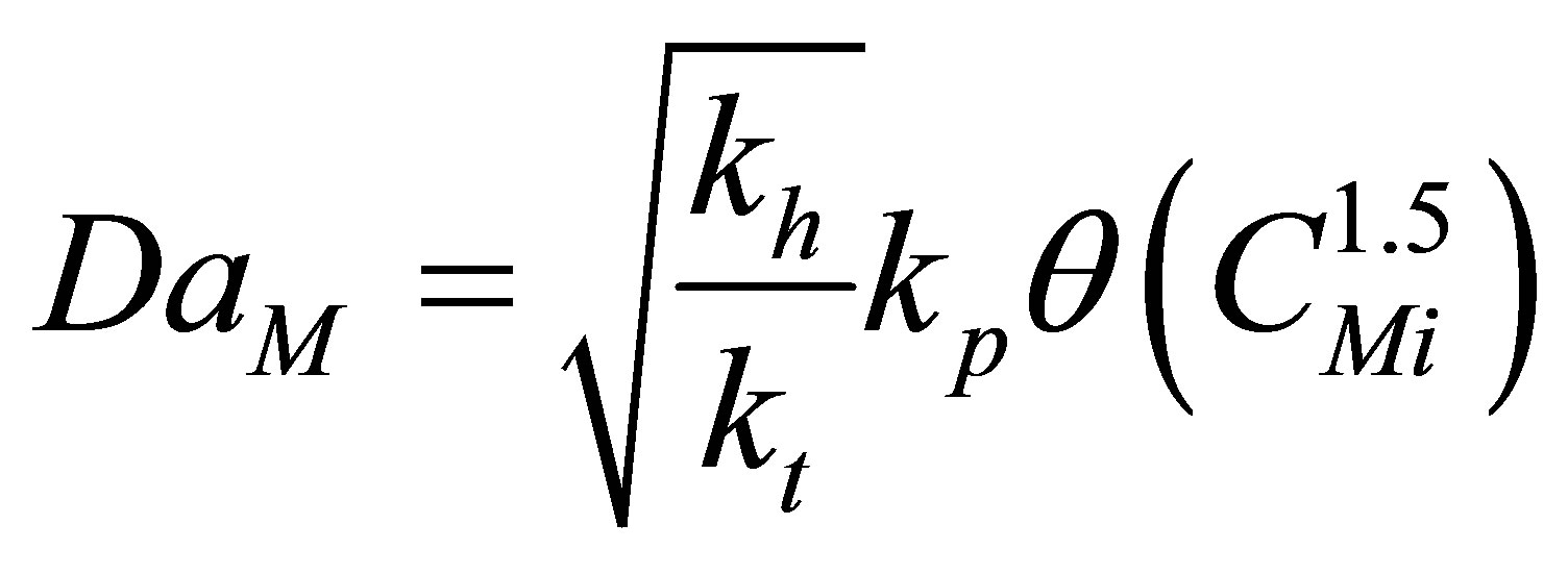 (65)
(65)
The dimensionless groups are introduced into Equation (62), Equation (62) can now be written as follows:
 (66)
(66)
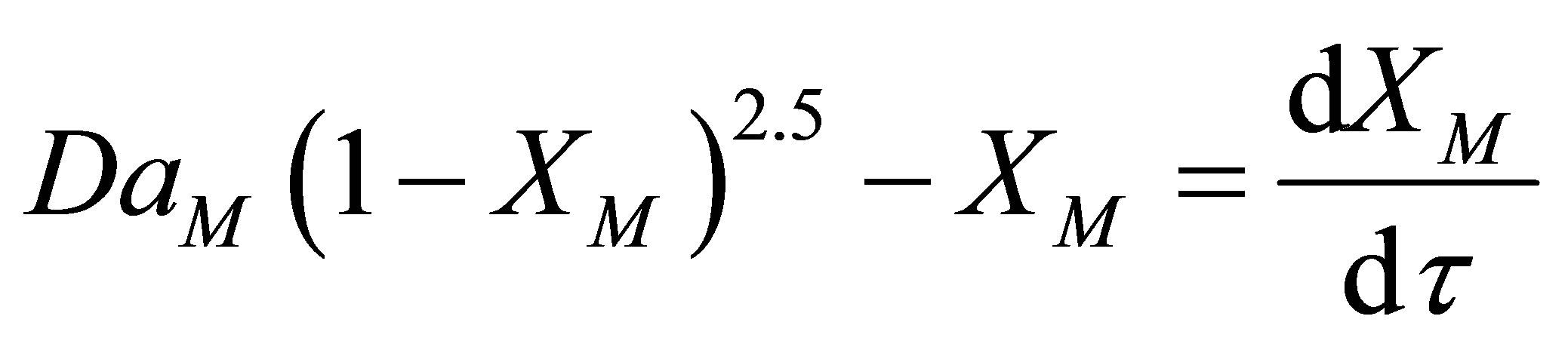
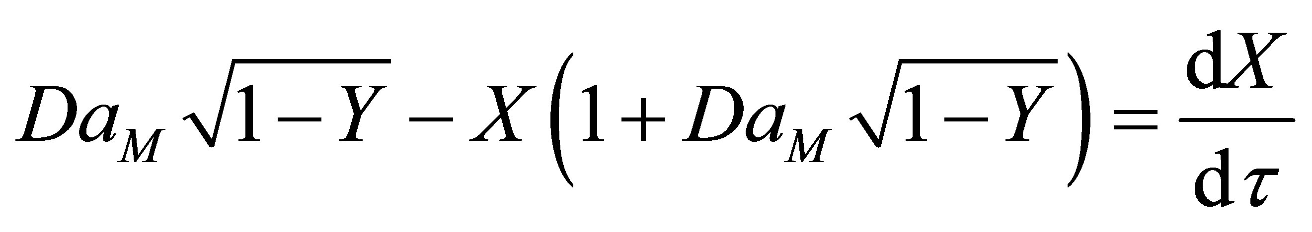
As the values of conversion of monomer, XM is less than 1, Binomial infinite series expansion can be a reasonable approximation for (1–XM)2.5. Higher order terms would be small. Truncation of terms higher than 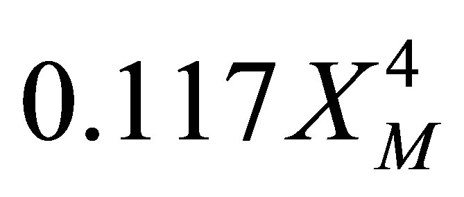 leads to:
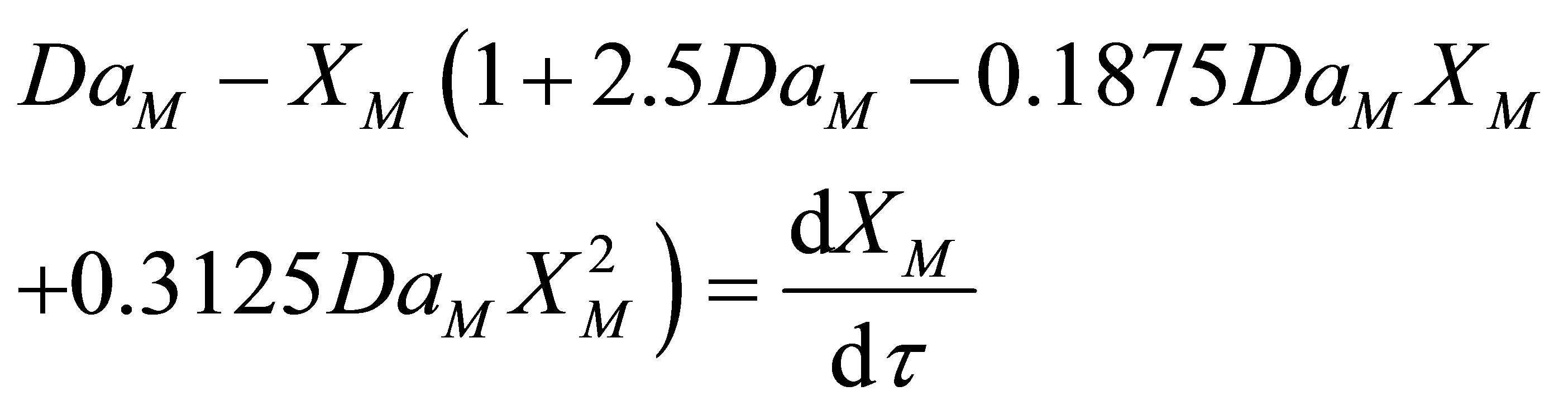 (67)
(67)
Equation (67) can be solved for by the method of superposition of the transient and the steady state solutions. Let,
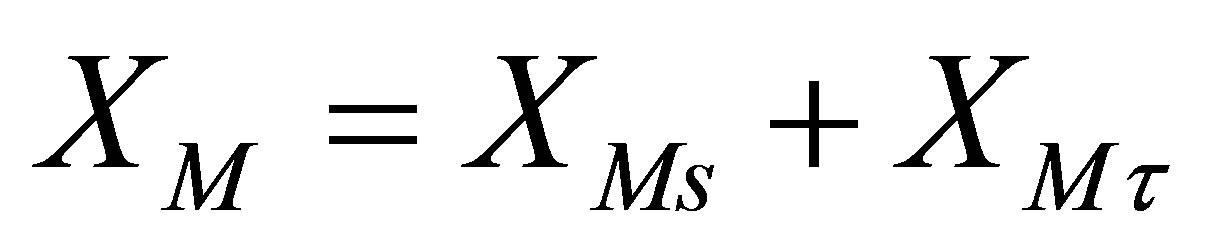 (68)
(68)
Equation (67) can be written as two separate equations: 1) one for the steady state component, XMs and; 2) transient state component, XMt.
 (69)
(69)
 (70)
(70)
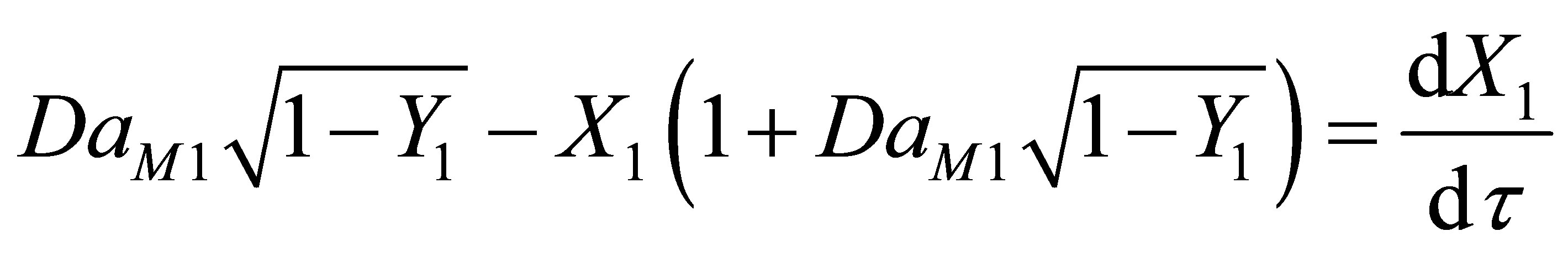
The equation for steady state conversion of monomer, Equation (69) was solved for by the method of Newton Raphson (Chapra and Canale, [14]) for finding the roots of the equation. The numerical solution was obtained using MS Excel 2007 for Windows on a desktop computer. Convergence for a considered Damkohler number was rapid. No multiplicity was found. The Damkohler number was varied and the result for each Damkohler number is shown in Table 1. This is also plotted in Figure 7. The steady state conversion XMs varies in a sigmoidal manner as a function of Damkohler number. For small Damkohler number the curvature is concave upward and changes to convex upward at large Damkohler numbers.
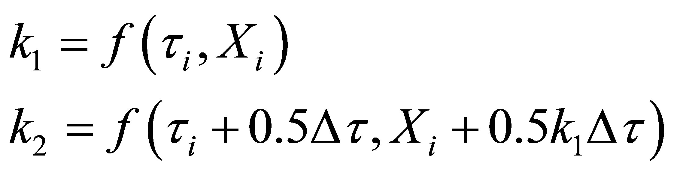
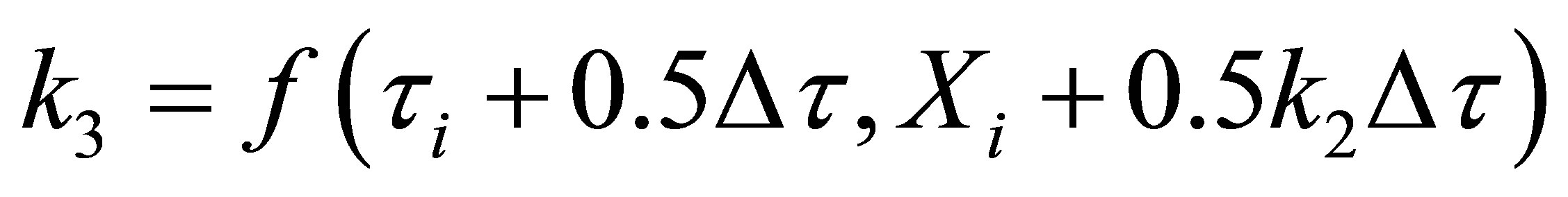
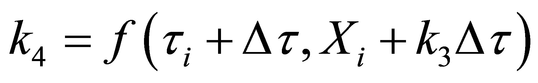
Equation (70) was integrated using fourth order RungeKutta method on a MS Excel 2007 spreadsheet for Windows on a desktop computer. The weigths used were as given in Chapra and Canale [14]. They are given here below:
 (71)
(71)
where,
Table 1. Steady state conversion for various values of DaM.
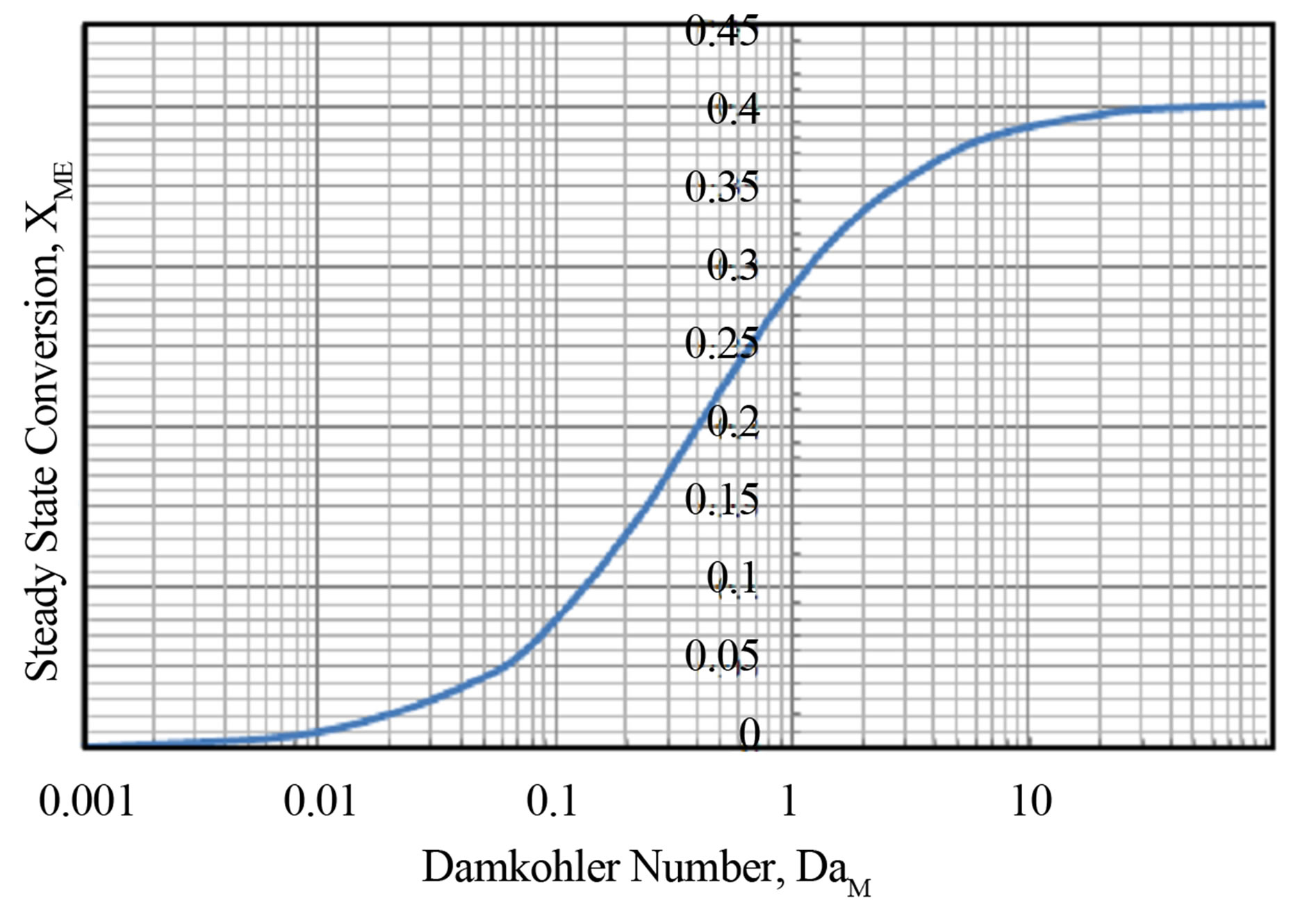
Figure 7. Steady state conversion as a function of Damkohler number.
 (72)
(72)
 (73)
(73)
 (74)
(74)
The transient conversion of the monomer as a function of dimensionless time is plotted in Figure 8 and Figure 9 for Damkohler numbers of 2 and 10.0. No multiplicities were found. The output response was monotonic. The transient conversion rises to a asymptotic steady state limit. Larger the Damkohler number the attainment of the asymptotic limit is rapid.
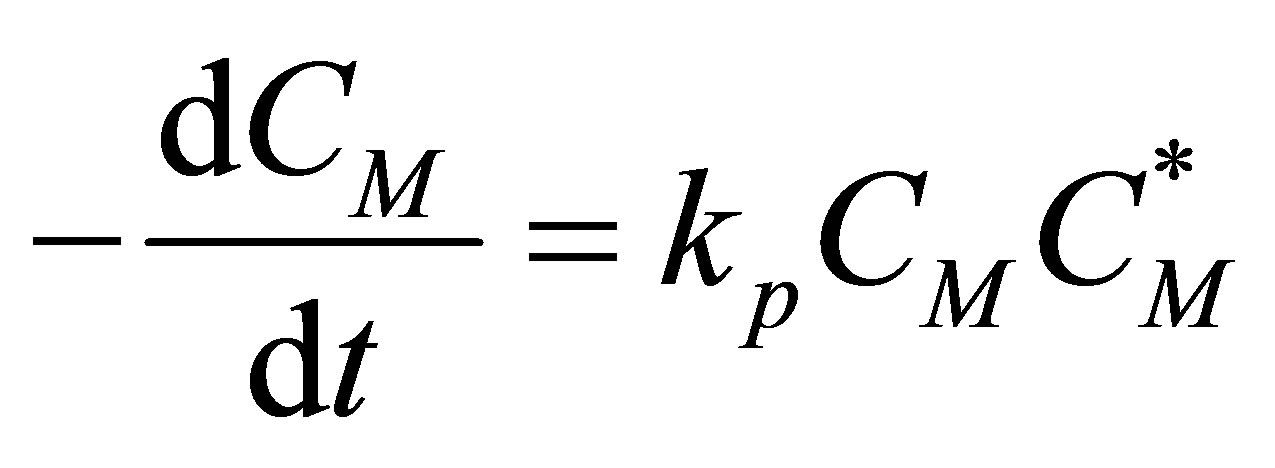
7.2. Transient Conversion during Initiation Polymerization in CSTR
Example 2:
Consider a CSTR (Figure 10) used for polymerization of styrene using a initiator such as TBPO, tertiary butyl peroxide. The free radical reactions can be represented by the following equations:
The polyrate of M is pseudo-first order and is given by:
Initiation
 (75)
(75)
Propagation
 (76)
(76)
Termination
 (77)
(77)
Assuming a pseudo-steady state, i.e. the initiator radicals will react as soon as they are formed:
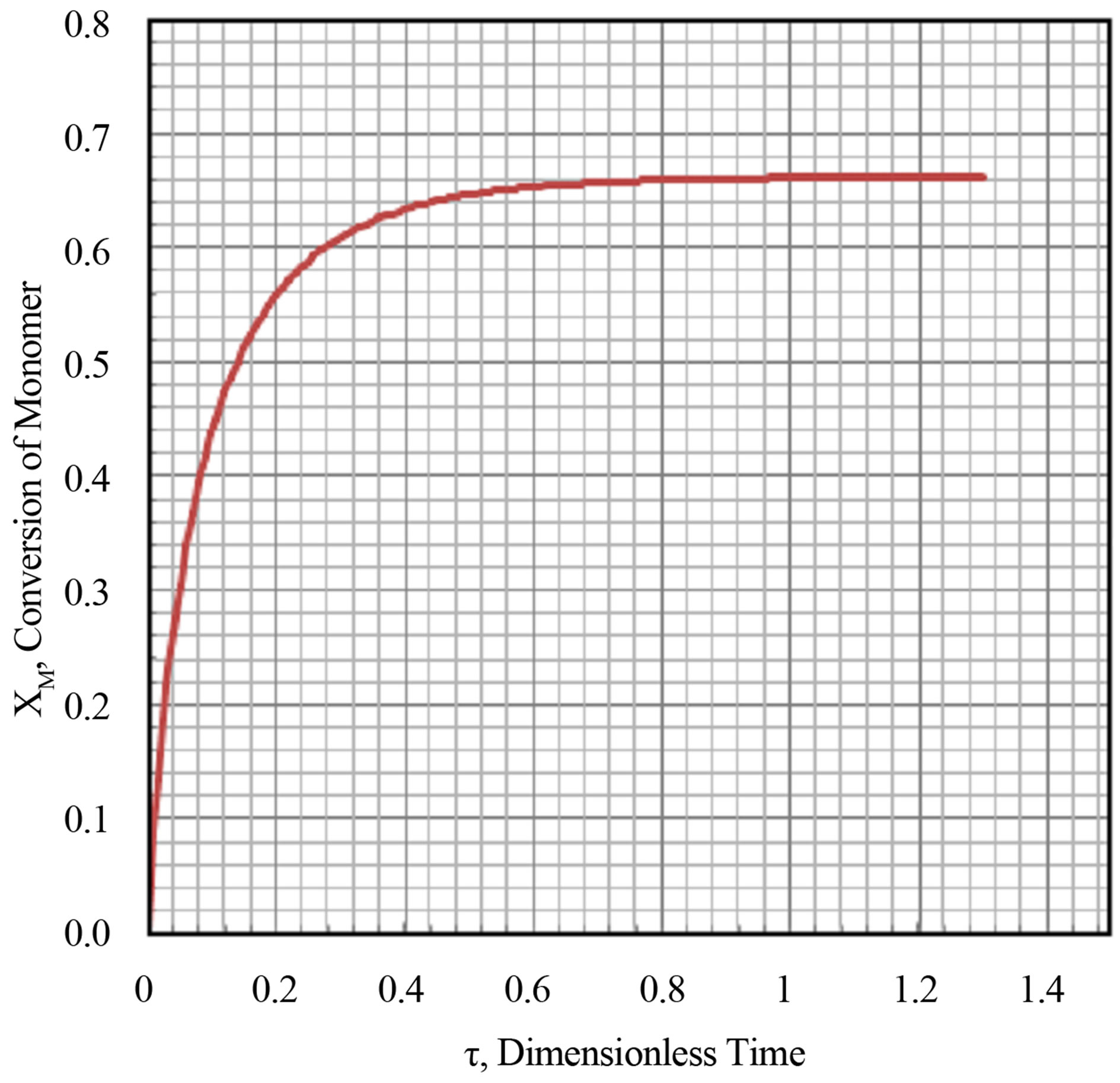
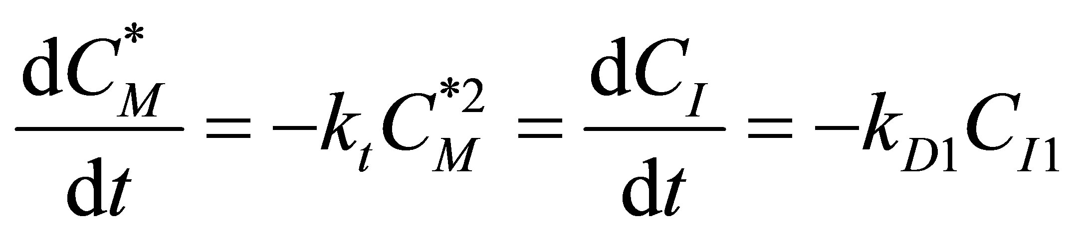
Figure 8. Transient conversion as a function of time at Da = 2.0.
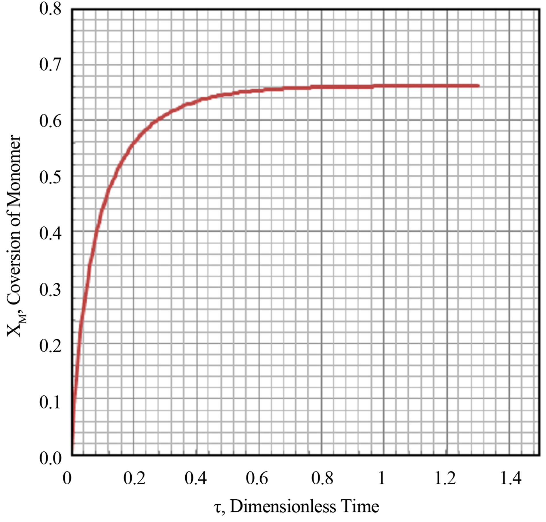
Figure 9. Transient conversion as a function of time at Da = 10.
 (78)
(78)
Or, (79)
(79)
Hence the rate of reactions can be written as one equation as;
 (80)
(80)
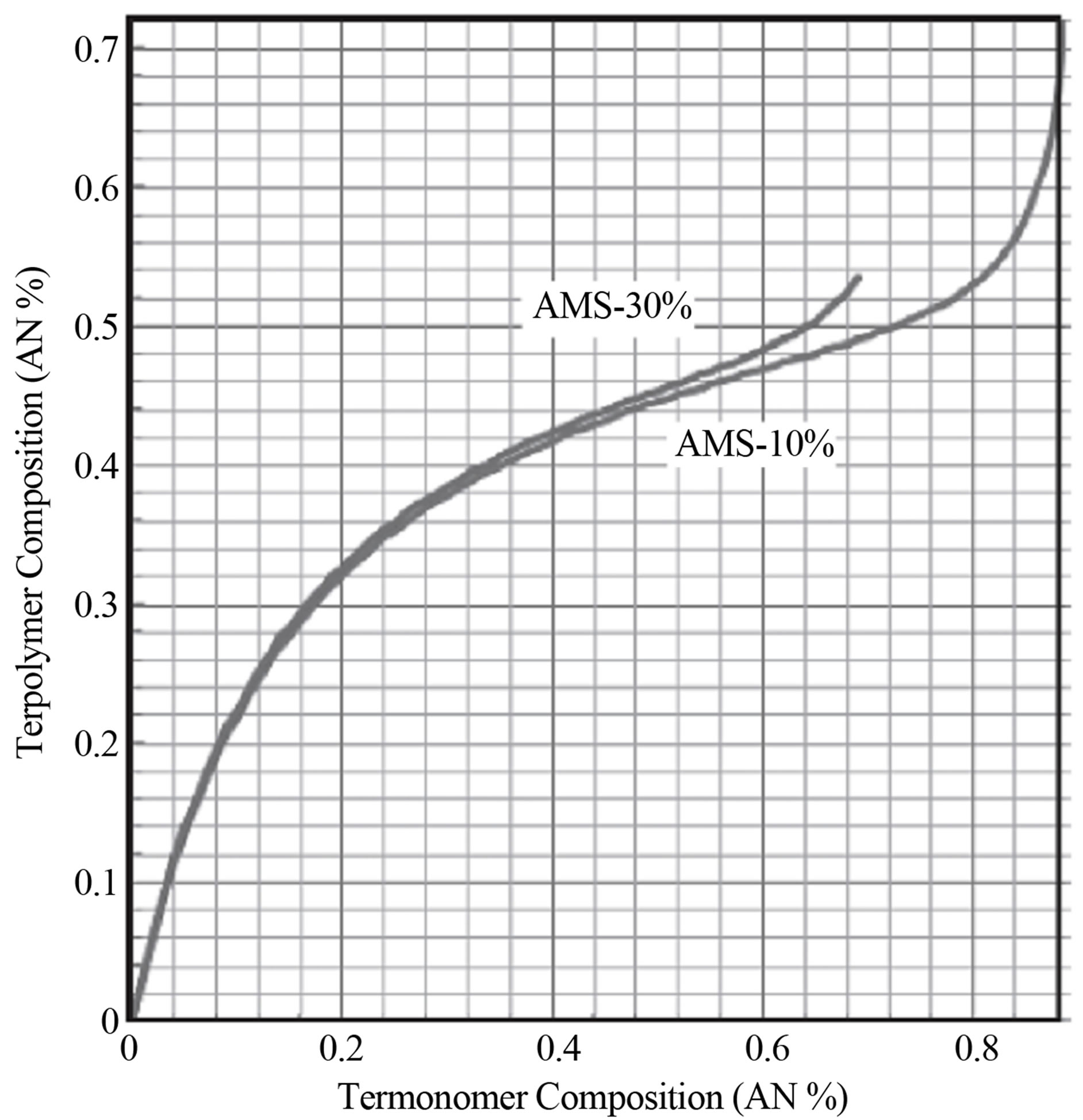
Figure 10. Terpolymer composition vs monomer composition for STY-AN-AMS system for two different compositions of AMS.
Obtain the model equations for the conversion of monomer, CM as a function of time with the given inlet monomer concentration of CM0 and initiator concentration. Assume that the flow is incompressible and the reactor volume remains a constant throughout the reaction. Discuss the transient behavior of the concentration of monomer in the kettle from the start-up of the reactor. Use the dimensionless group Damkohler number if necessary.
The CSTR reactor volume is considered as the control volume. The component mass balances for the initiato concentration, CI can be written as follows:
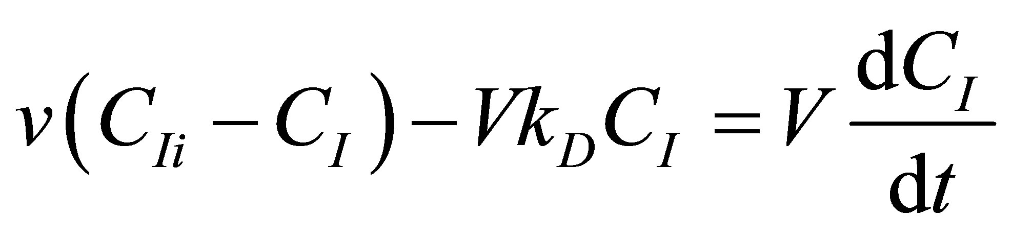 (81)
(81)
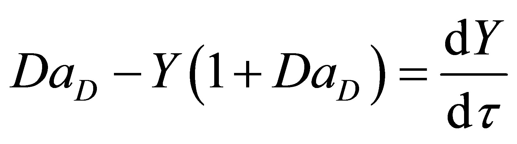
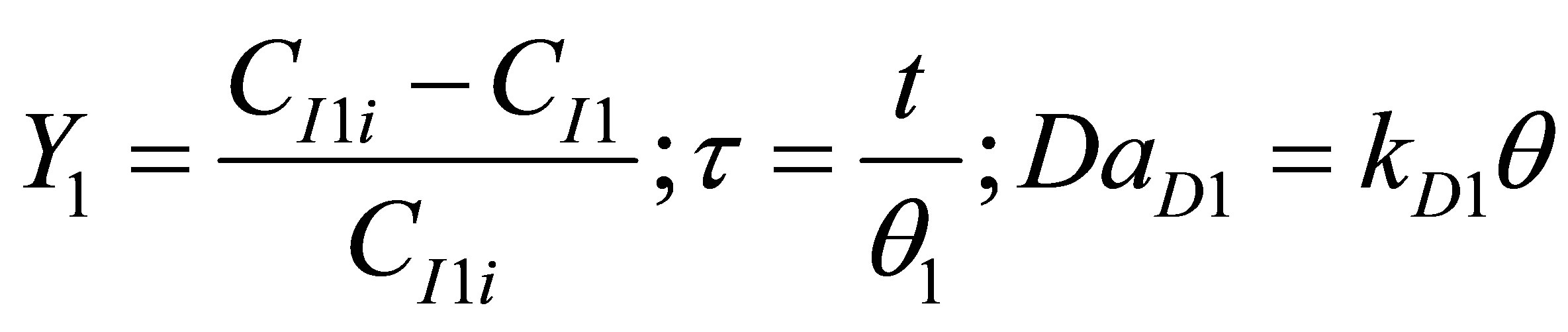
Let the conversion of the initiator be Y and dimensionless time by t and Damkohler number (dissociation) be DaD as given by:
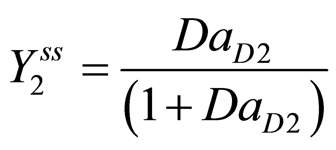
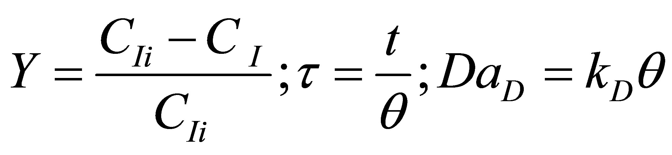 (82)
(82)
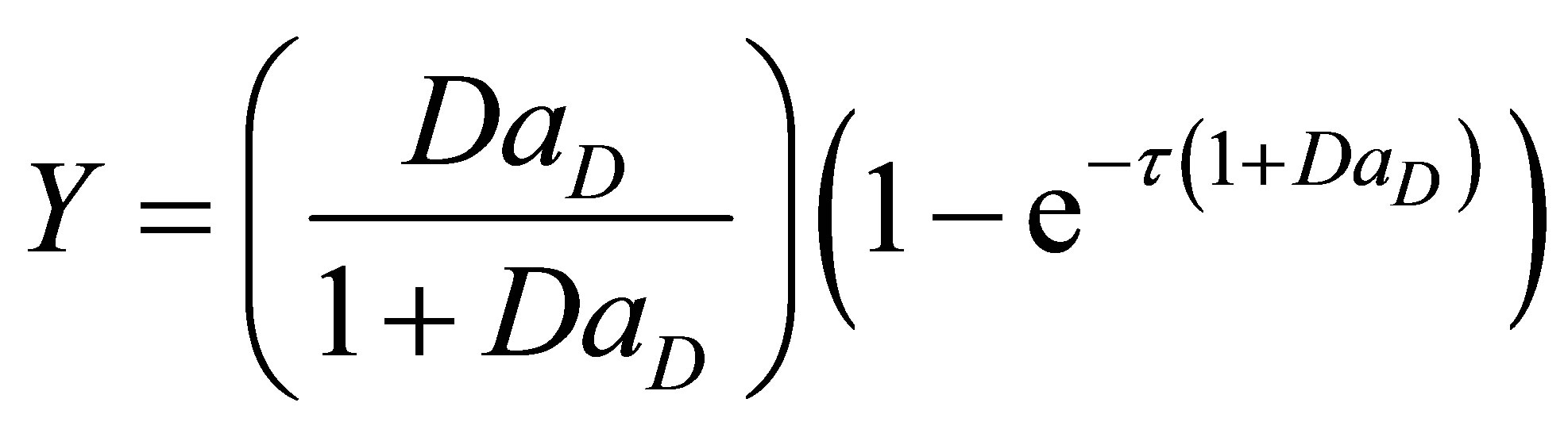
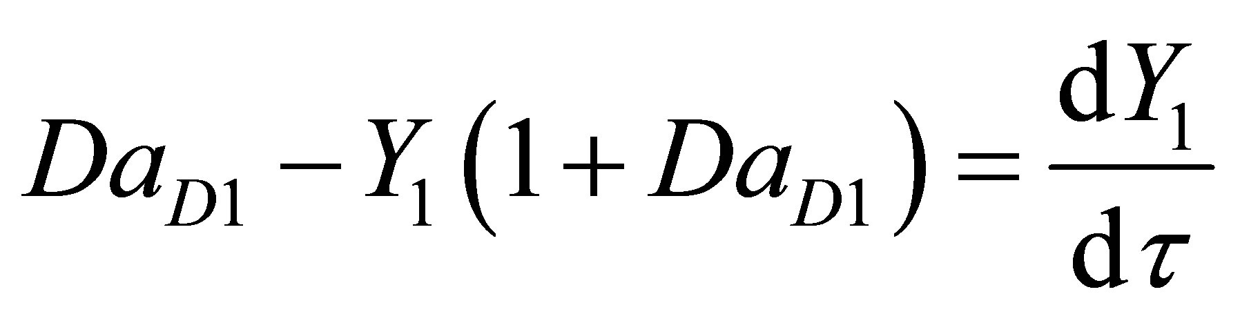
where, q is the residence time of the reacting species in the reactor. Equation (81) then becomes:
 (83)
(83)
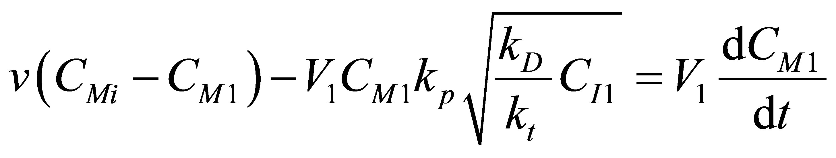
The component mass balances for the monomer concentration, CM can be written as follows:
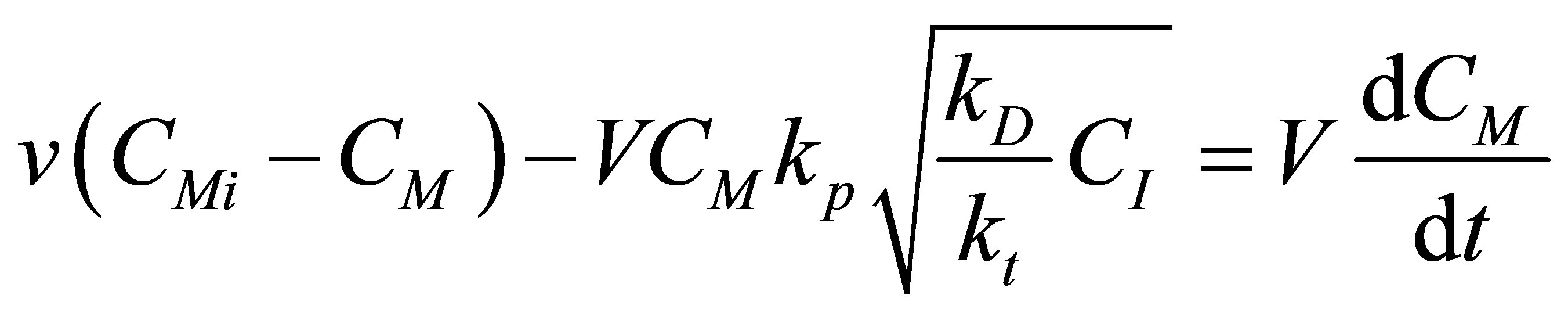 (84)
(84)
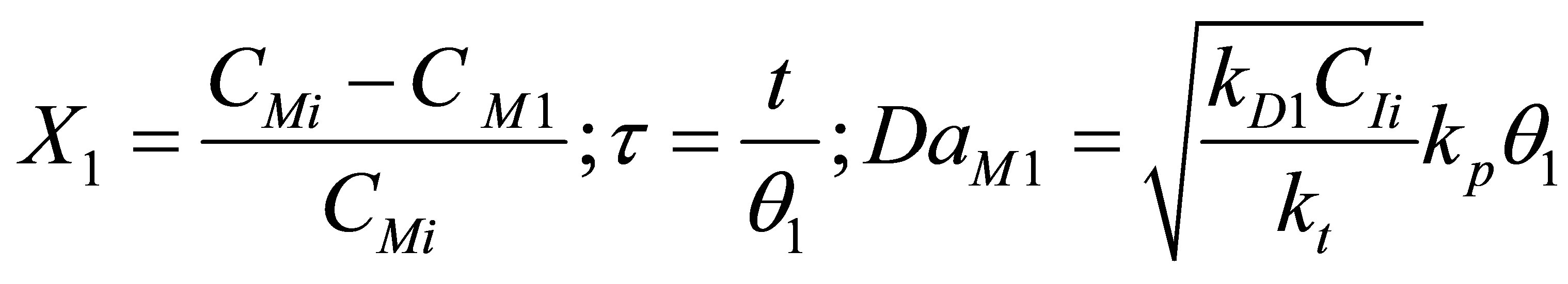
Let the conversion of the monomer be X and dimensionless time by t and Damkohler number (monomer) be DaM as given by:
 (85)
(85)
where, q is the residence time of the reacting species in the reactor. Equation (84) then becomes:
 (86)
(86)
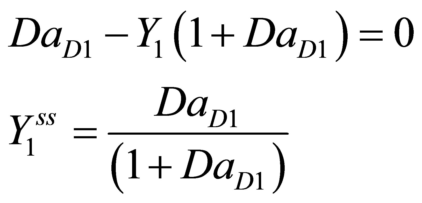
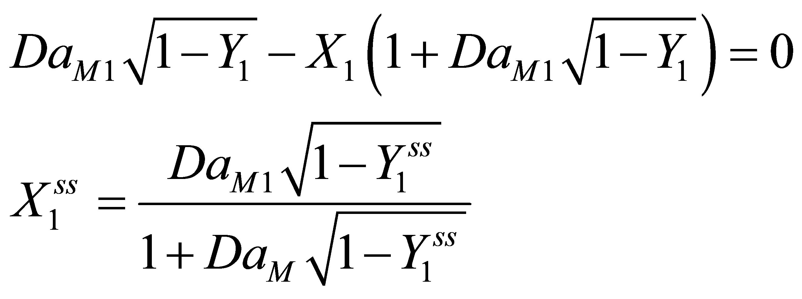
At steady state Equation (86) and Equation (83) becomes:
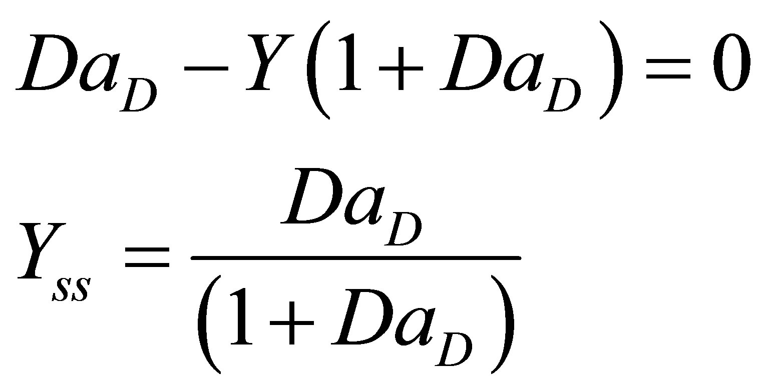 (87)
(87)
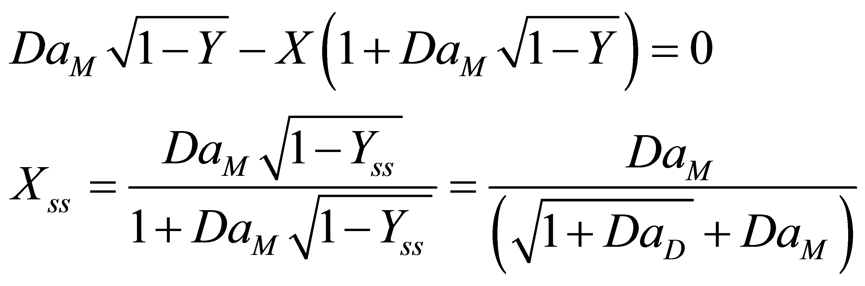 (88)
(88)
There were no multiplicities found in the expression for steady state conversion of initiator and monomer. Equation (88) is non-linear. Equation (88) can be integrated by separation of variables and the model solution seen to be;
 (89)
(89)
Equation (86) was solved using the fourth order RungeKutta method [14]. The parameters used and calculated in the simulation are given in Table 2.
The transient conversion of monomer was computed and plotted in Figure 11 along with the transient conversion of initiator from Equation (83). It can be seen from Figure 9 for the parameters used in the simulation study the transient conversion of monomers undergoes a maximum value. Multiplicity can be seen in the transient conversion of monomer X, especially near the maxima. The simulation was conducted using a MS Excel 2007 for Windows on a desktop computer.
The maximum transient conversion of monomer X for the parameters used in the simulation study was found to be 0.902. An example of multiplicity is at transient conversion of monomer X = 0.88. There are two dimensionless times associated with this conversion. These can be seen from Figure 3.9 to be t = 0.19 and t = 0.8. The reason for the occurrence of maxima is not clear. The scheme of free radical reactions does not have a reverseble step. There is a decrease in monomer conversion after a said time.
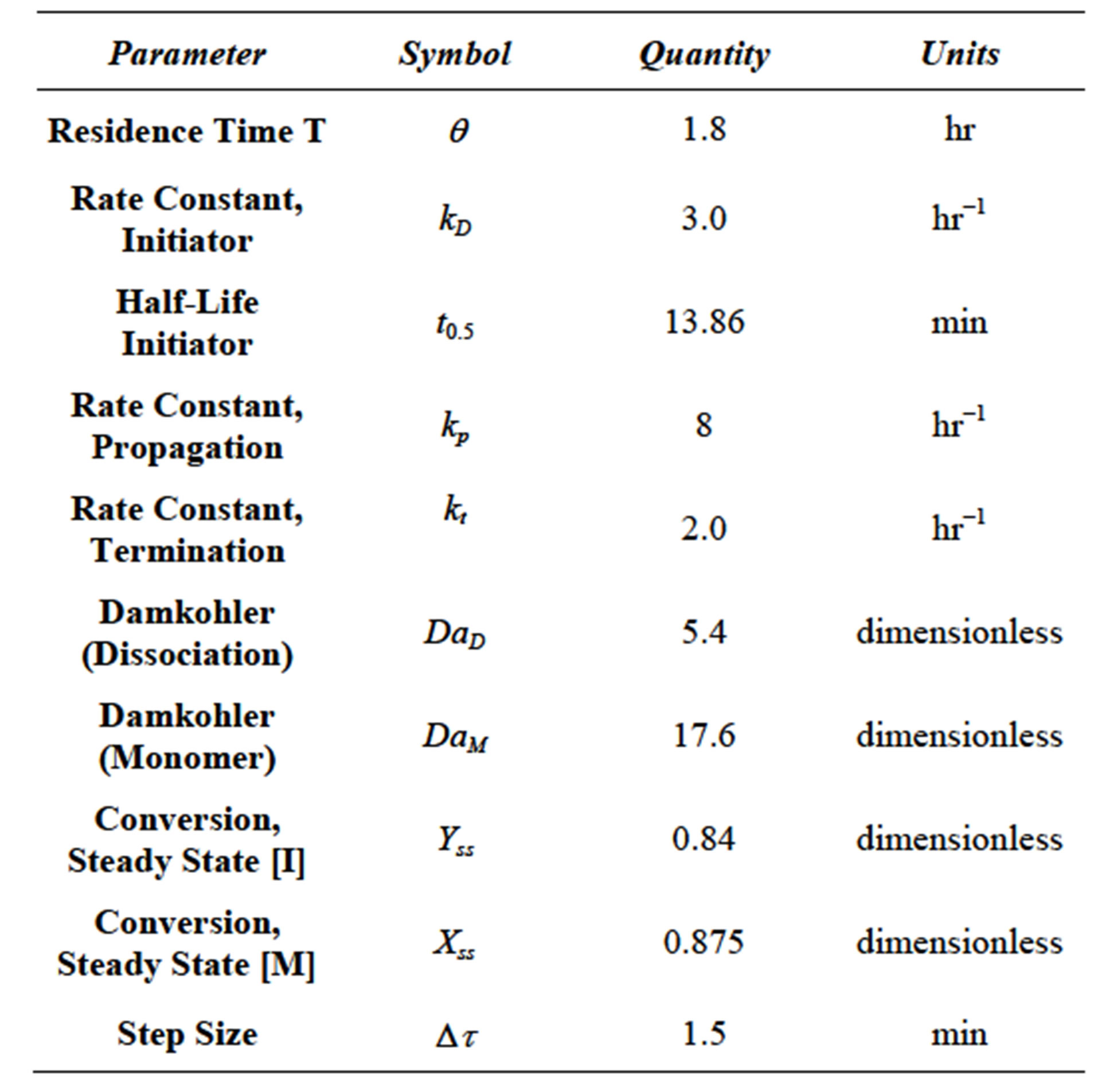
Table 2. Parameters used during simulation of monomer and initiator.
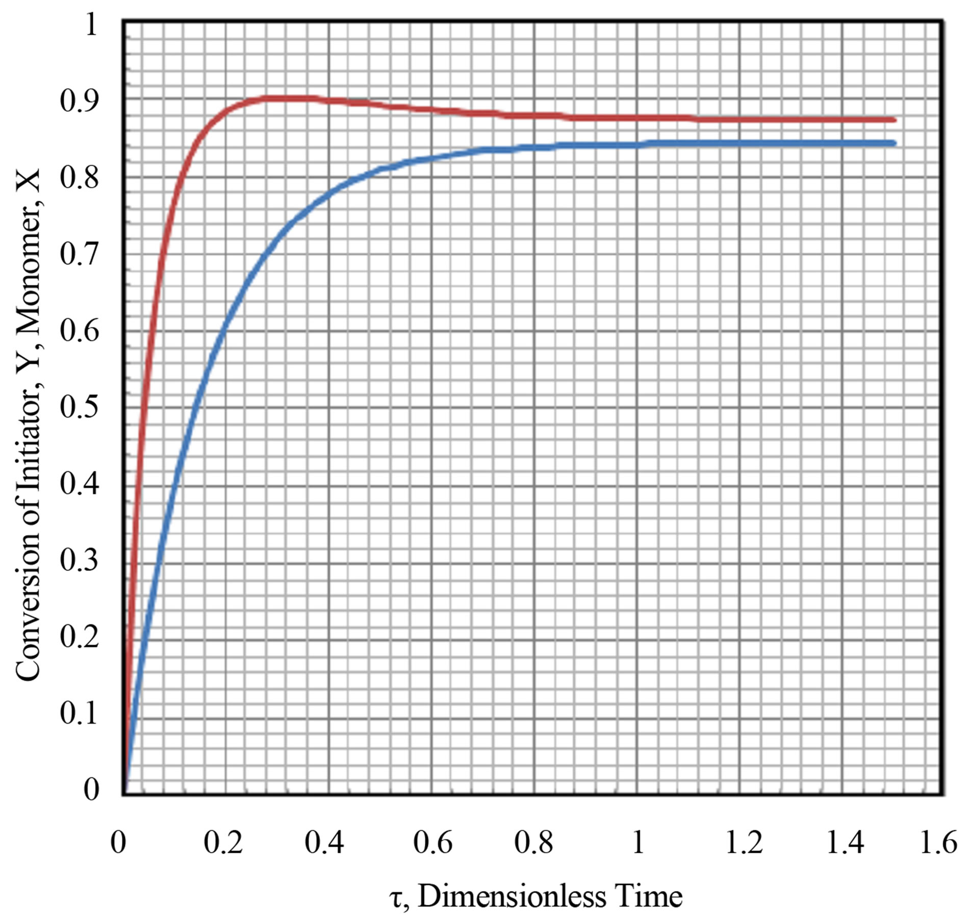
Figure 11. Transient conversion of monomer X and initiator Y.
7.3. Transient Conversion in Two CSTRs in Series—Initated Case
Example 3
The initiation polymerization described in Example 3 is performed in two CSTRs in series (Figure 12). The volumes of the two reactors are constant during the polymerization reaction and are V1 and V2. Monomers such as styrene, acrylnitrile. Methyl methacrylate etc can be polymerization in this manner. Two initiators are used. Initiator type used is from the peroxy family. Examples
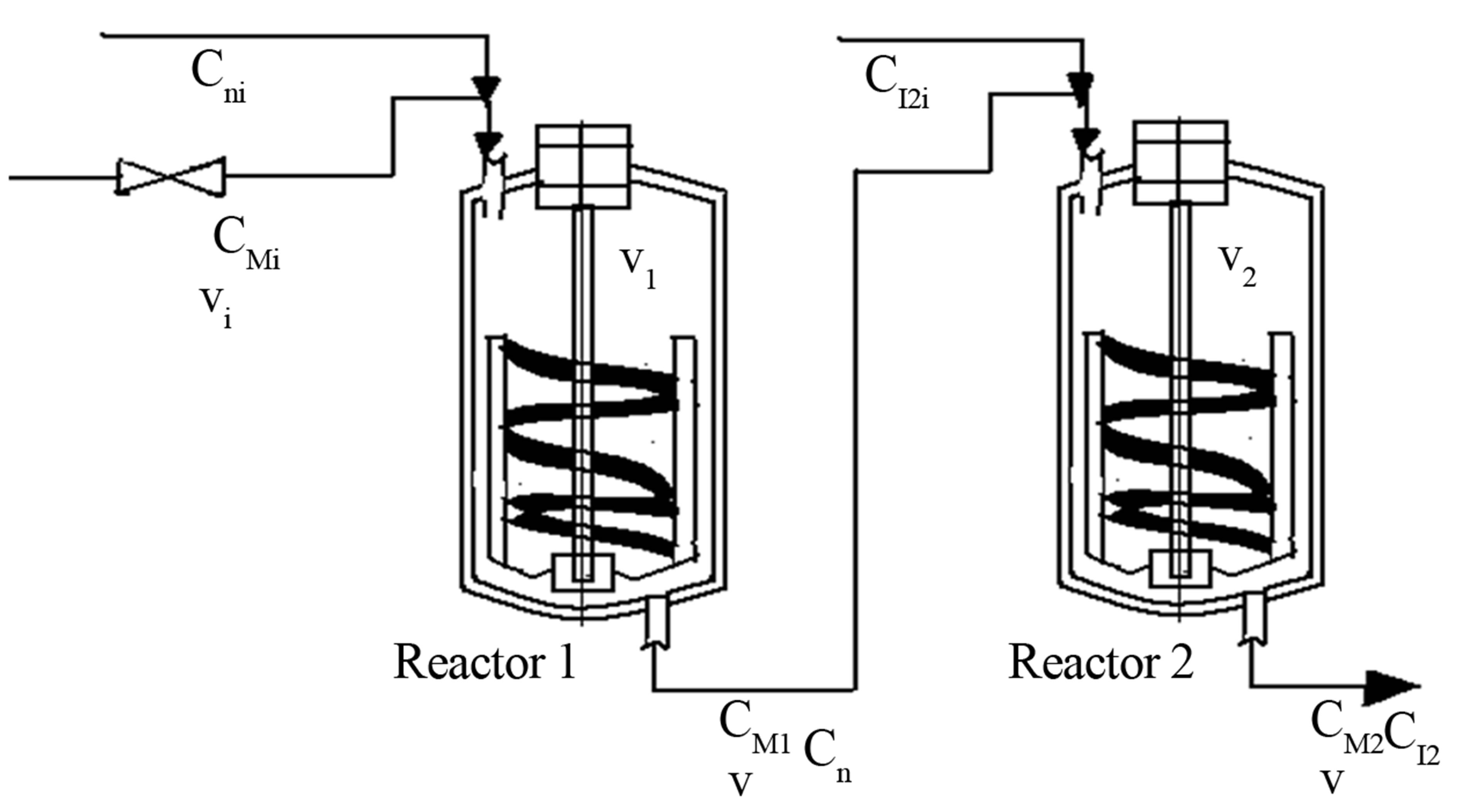
Figure 12. Initiation polymerization conducted in two CSTRs in series.
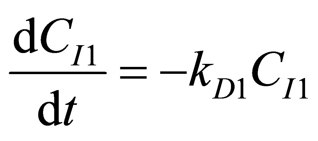
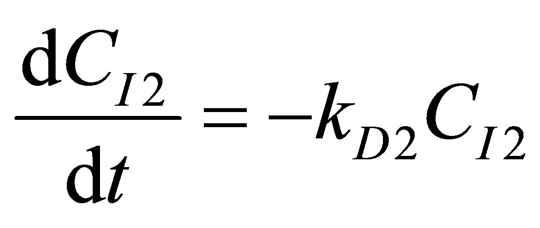
are TBPO, tertiary buty peroxide, TBPOND, tertiary butyl peroxy neodeconoate or TBPP, tertiary butyl peroxy pivalate. The two reactors are operated at different temperatures. The second reactor temperature is higher than the first reactor temperature. The initiator selected for use in second reactor is by calculation of half-live of the initiator at reactor temperature. The monomer concentrations at the exit of the two reactors R1 and R2 are CM1 and CM2 respectively. The initiator used in R1 is I1 and has a inlet concentration of CI1i and the efflux concentration of CI1. The initiator used in R2 is I2 and has a inlet concentration of CI2i and the efflux concentration of CI2. The two CSTRs are operated in series and are well agitated. In order to handle viscous polymer syrups the helical ribbon agitators are used as shown in Figure. Obtain the output response for the initiator and monomer from R1 and R2.
The polyrate of M is pseudo-first order and is given by:
Initiation (R1)
 (90)
(90)
Initiation (R2)
 (91)
(91)
Propagation
 (92)
(92)
Termination
 (93)
(93)
Assuming a pseudo-steady state, i.e. the initiator radicals will react as soon as they are formed:
 (94)
(94)
Or, 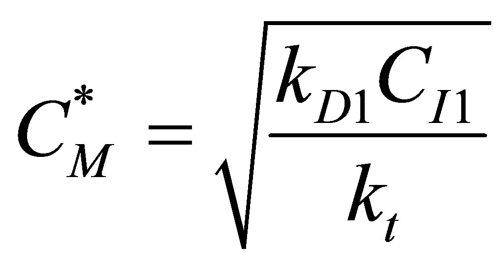 (R1) (95)
Hence the rate of reactions can be written as one equation as:
 (R1) (96)
 (R2) (97)
The CSTR reactor volume is considered as the control volume. The component mass balances for the initiator concentration, CI1 can be written as follows for the first CSTR, R1 as:
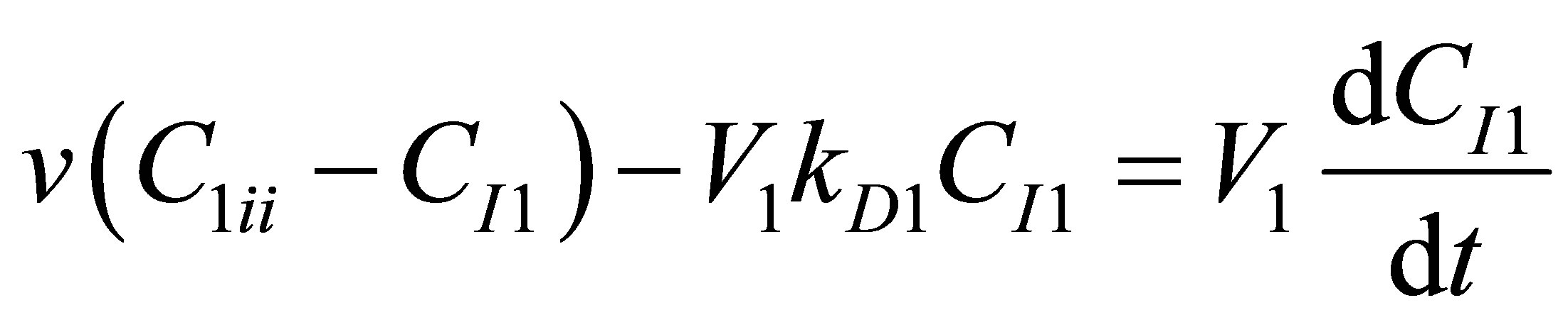 (98)
(98)
Let the conversion of the initiator be Y and dimensionless time by t and Damkohler number (dissociation) be DaD as given by:
 ; (99)
where, q1 is the residence time of the reacting species in R1 Equation (98) then becomes;
 (100)
(100)
The component mass balances for the monomer concentration, CM can be written as follows;
 (101)
(101)
Let the conversion of the monomer be X and dimensionless time by t and Damkohler number (monomer) be DaM as given by;
 (102)
(102)
where, q1 is the residence time of the reacting species in th reactor. Equation (101) then becomes;
 (103)
(103)
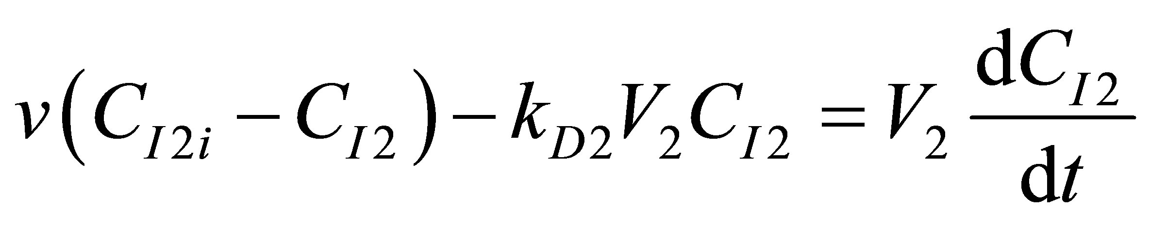
The component balance for the initiator I2 into the second reactor and the monomer that is further converted in R2 can be written as follows:
 (104)
(104)
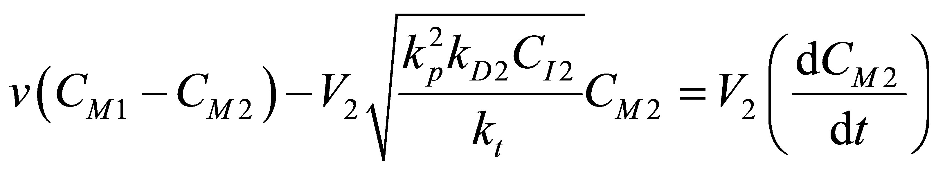 (105)
(105)
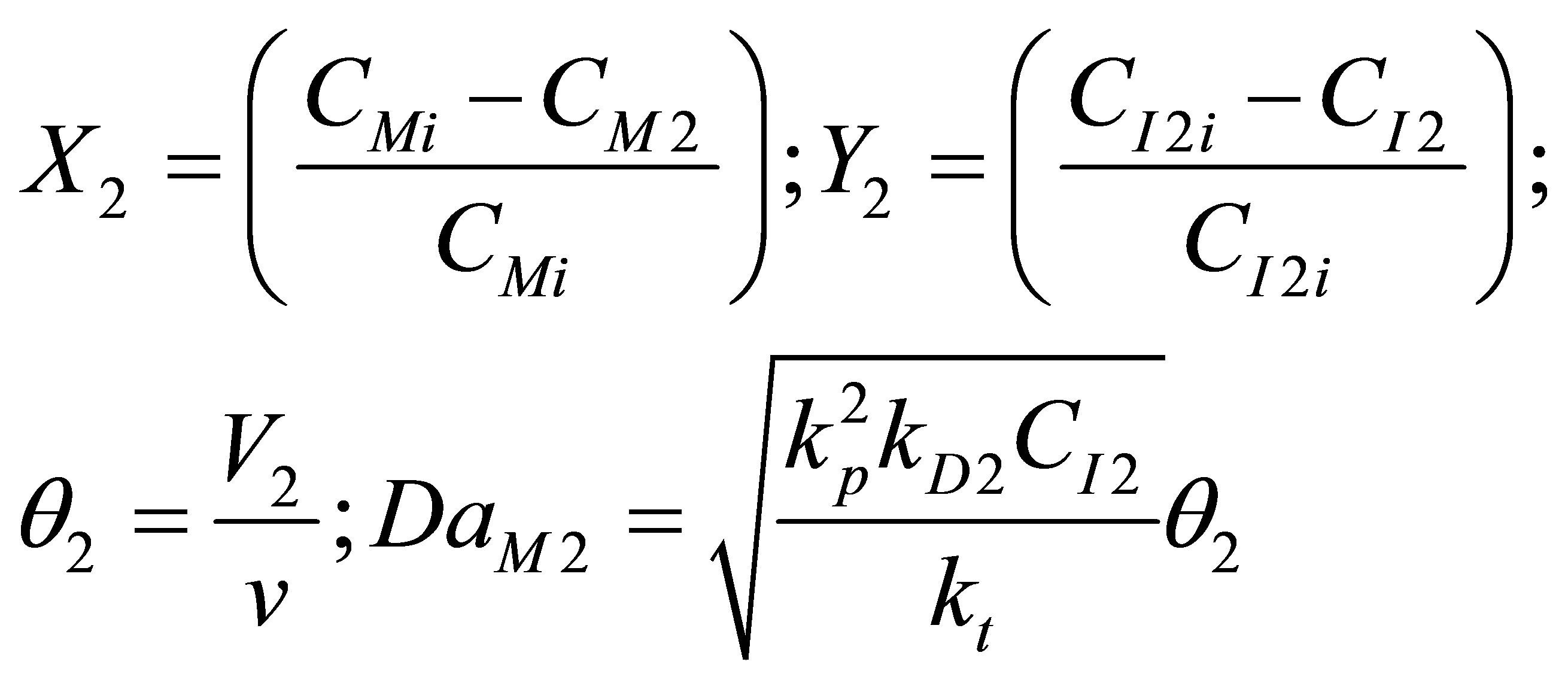
The dimensionless variables and parameters as follows:
 (106)
(106)
Equations (104) and (105) become on non-dimensionalization:
 (107)
(107)
 (108)
(108)
At steady state Equations (103) and (108) become:
 (109)
(109)
 (110)
(110)
 (111)
(111)
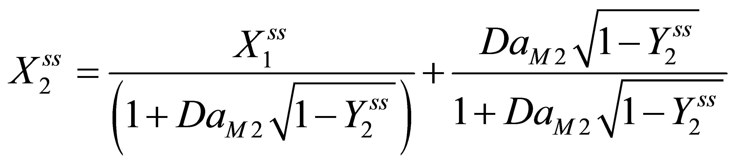 (112)
(112)
Integrating Equation (107) upon separation of variables:
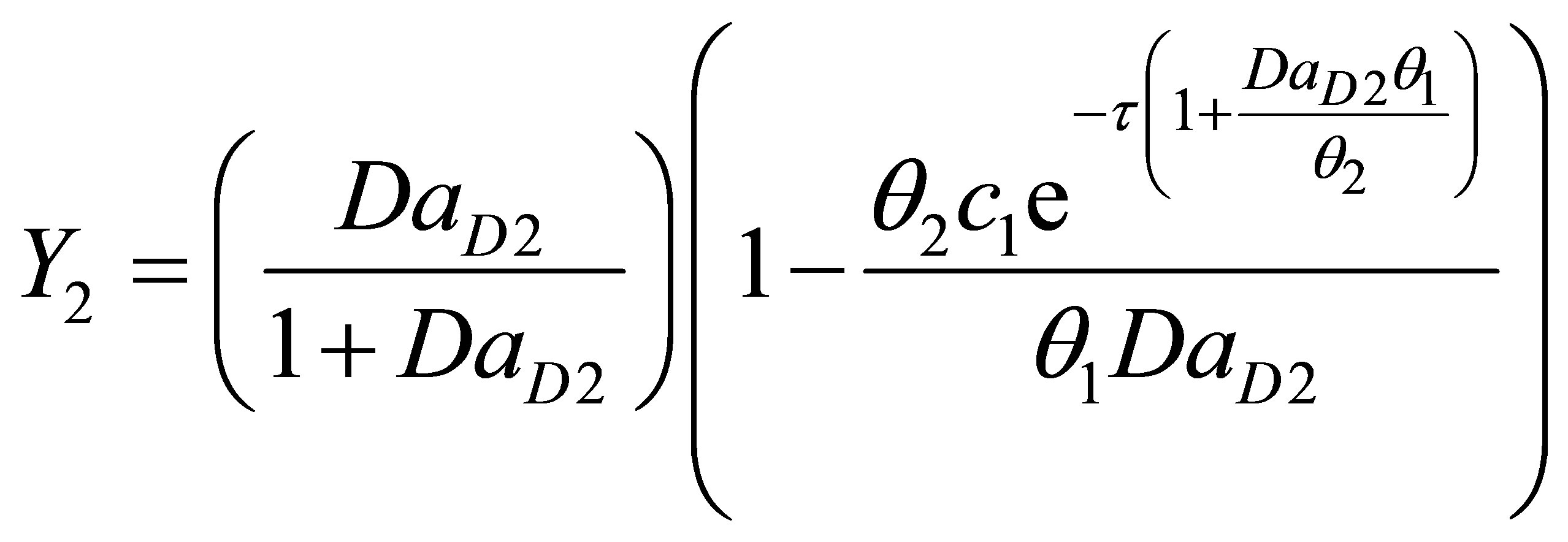 (113)
(113)
The integration constant c1 can be solved for from the initial condition:
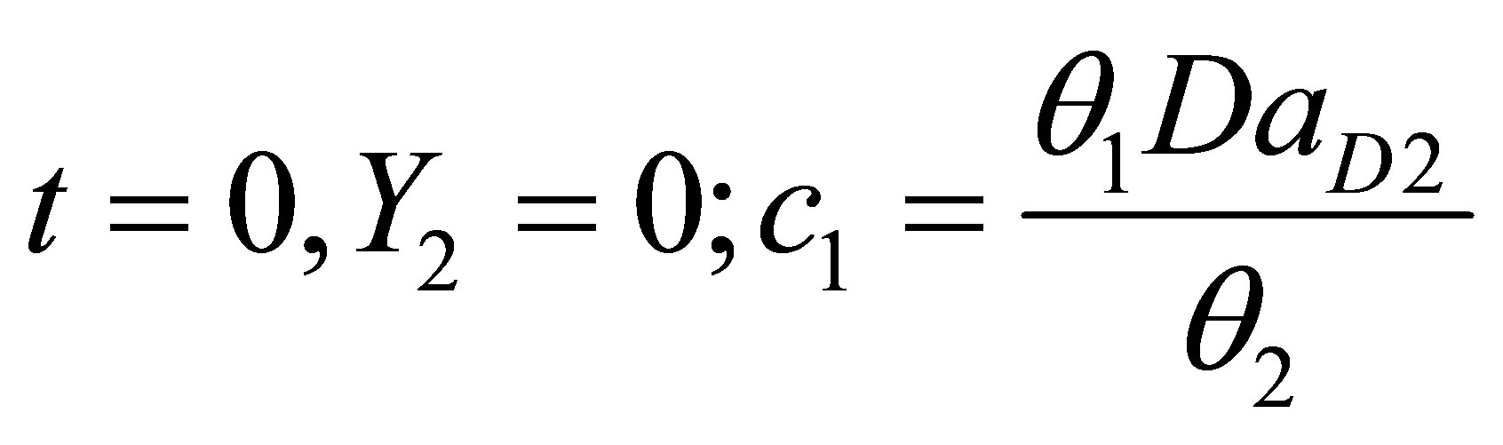 (114)
(114)
Equation (113) becomes:
 (115)
(115)
Equations (103) and (108) were integrated using Runge Kutta fourth order method. The equations are nonlinear. The weights used are given in Equations (71)-(74). The numerical integration was carried forward using MS Excel 2007 for Windows in a desktop computer. The results are shown in Figure 13. The parameters used in the simulation are listed in Table 3. As can be been from Figure 12 multiplicity can be seen in conversion of monomer in R2. No multiplicity can be seen in conversion fo monomer in R1. The initiator response in R2 was slower than the the initiator response in R1. The conversion achived in R1 was lower compared with the set of conditions seen in Example 2.0.
8. Conclusions
1) Composition of a random, copolymer can be calculated as a function of comonomer compositions and reactivity ratios when made in a CSTR by free radical polymerization methods at a suitable temperature and with an initiator. QSSA, quasi steady state approximation was used in the analysis. Copolymerization composition equation is given by Equation (6) for a system with two comonomers. The relation between copolymer composition and comonomers’ composition for a two component copolymer is given by Equation (10). This can be included in the single compartment pharmacokinetic model.
2) The copolymer composition as a function of comonomer compositions are shown in Figure 1 for reactivity ratio values of r21 0.02, 0.04, 0.1, 0.1, 1, 2, 4 and 16 holding r12 constant. When two reactivity ratios r12 = r21 = 0 the copolymer is expected to result in alternating microstructure. Copolymerization is said to be ideal when during formation the reactivity ratios r12 = r21 = 1. Block architecture results when one of the reactivity ratios is much greater than the other. Azeoptropic composition is when copolymer composition equal to the comonomer composition.
3) Copolymer composition curve for AMS-AN copolymers as a function of comonomer compositions are presented in Figure 2 as an example of when one of the comonomers has a lower ceiling temperature. Two curves can be seen in Figure 2. One is without the ceiling temperature effect and the other is with the ceiling temperature effect. For AMS-AN copolymer, when the ceiling temperature effect is expected the AN-AN triads, tetrads, pentads and hexads can be expected to form in the product at higher concentrations.
4) For the case of terpolymer, the composition ratios of the product are presented as a function of comonomer ratios in Equations (18) and (19). The relations are functions of six reactivity ratios, r12, r21, r13, r31, r23 and r32 and ratios of comonomer compositions.
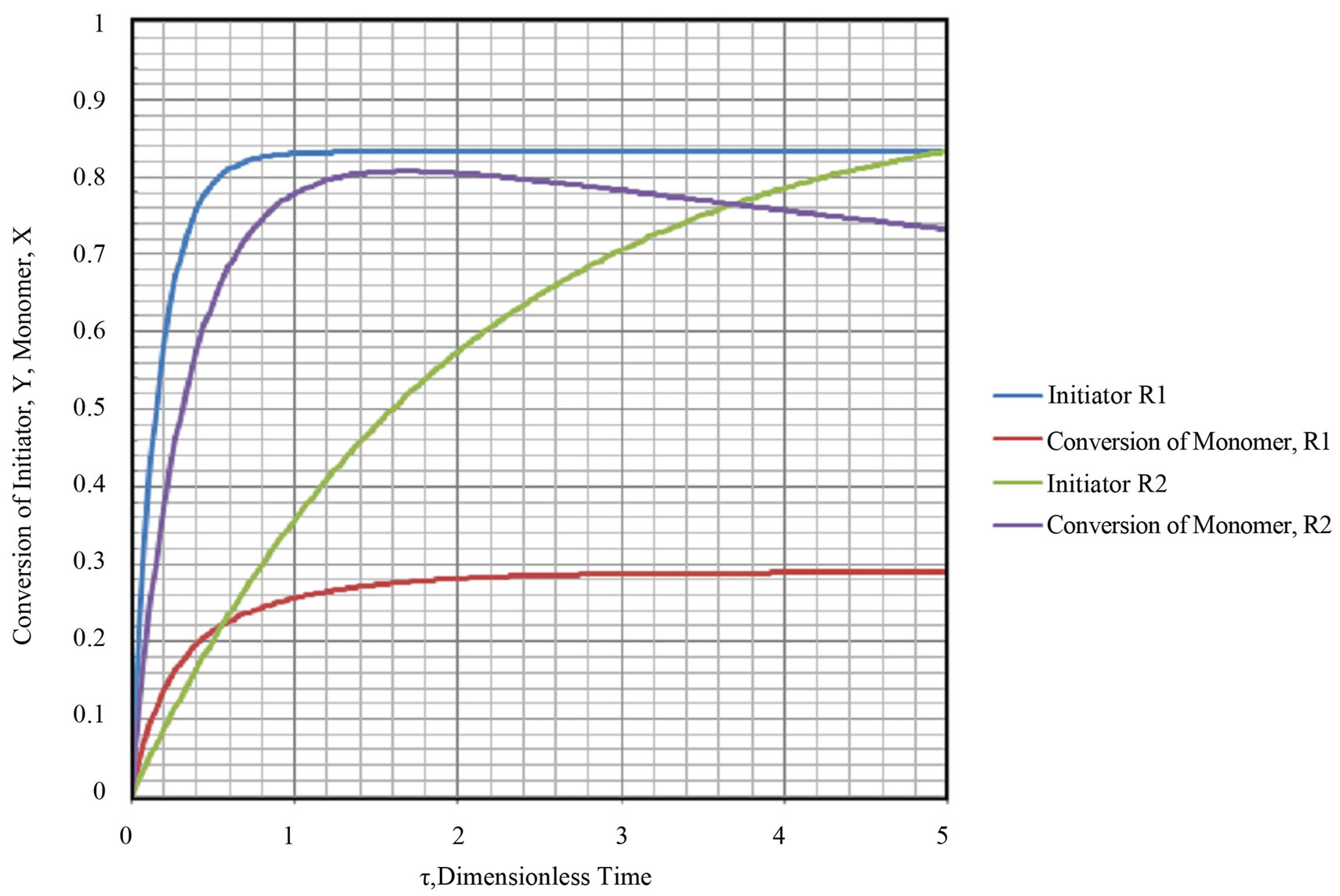
Figure 13. Output response of initiator and monomer from R1 and R2.
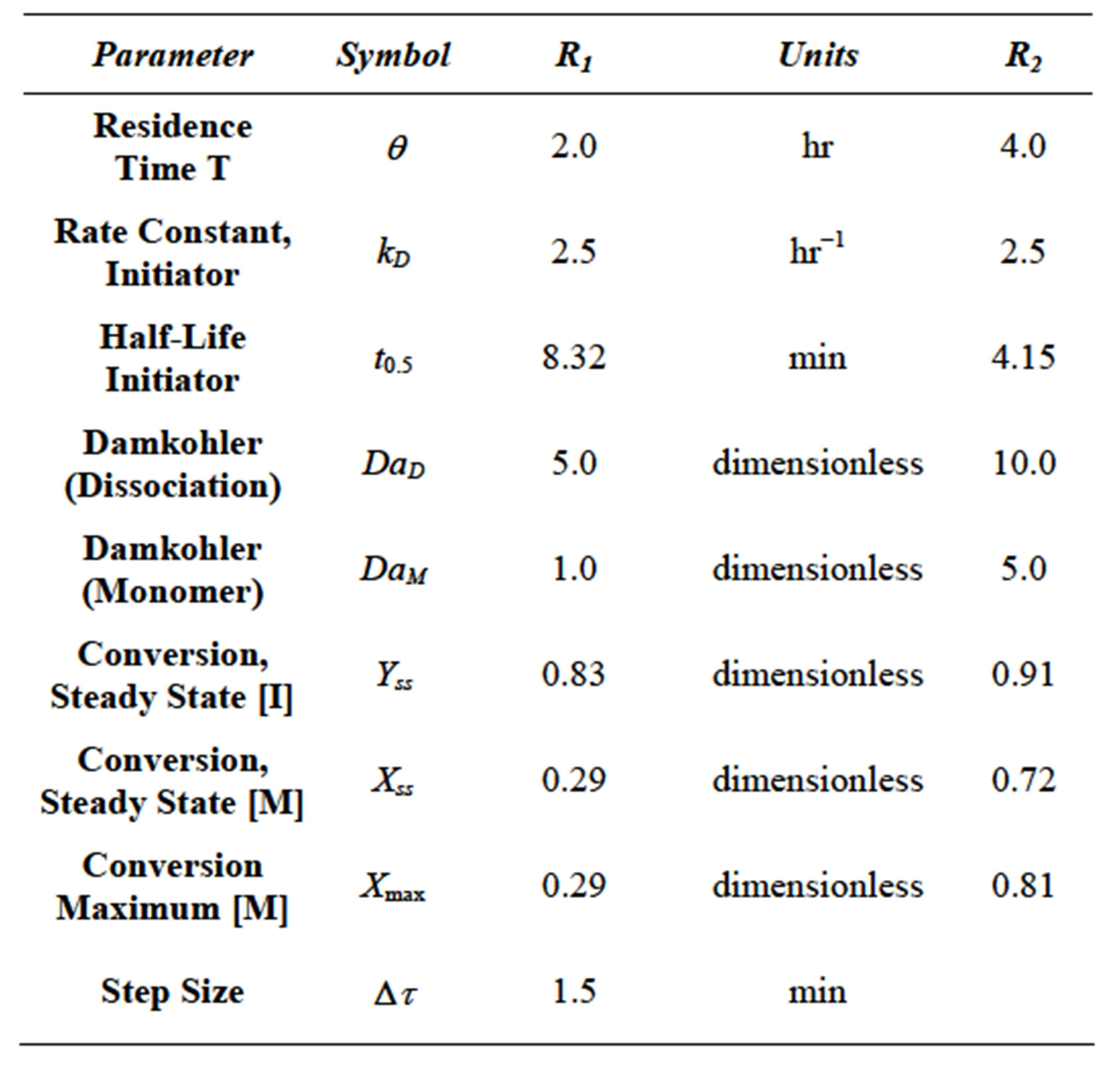
Table 3. Parameters used during simulation of monomer and initiator in 2 CSTRs in series.
5) A particular case of Equation (10) when r12 is 1 is given by Equation (22). The inverse problem of finding monomer composition for a desired polymer composition, i.e., expression of comonomer composition f1 in terms of copolymer composition, F1 results in a quadratic equation. Multiple real roots are found for certain values of compositions. An example is shown in Figure 3 for the case of DEF-AN, diethyl fumrate and acrylonitrile system. For copolymer composition range from F1 = 0.15 - 0.48 for a selected copolymer composition, two comonomer compositions can be seen from the model solution. Which one the CSTR is operated under is not clear. The two products at the same copolymer composition will have two different sequence distributions.
6) MAN-Styrene copolymer composition as a function of comonomer composition is given in Figure 4 as an example of a system with equal reactivity ratios, i.e., r12 = r21 = 0.25.
7) Terpolymer composition as a function of comonomers’ composition for Styrene-AN-AMS system at two different compositions of AMS is shown in Figure 5.
8) Methodology for calculation of copolymer composition has been extended to case of n monomers. The copolymer rate equation for n comonomers made in a CSTR in state space form is given by Equation (31). QSSA in state space form is given by Equation (35). Eigenvalues can be calculated from Equation (36). For some values of eigenvalues, sub critical oscillations in product can be expected. The model results can be included in the single compartment pharmacokinetic model.
9) Steady state and transient state conversion for initiated case and thermal case for 1 CSTR and 2 CSTRS were calculated and plotted in Figures (7)-(9) and 12. No multiplicity was found in the thermal case for 1 CSTR in the dynamics of transient monomer conversion.
10) Multiplicity was found in the initiated case for 1 CSTR in the dynmaics of transient conversion of monomer. The multiplicity was found in the second CSTR for the case of 2 CSTRs in series. No multiplicity was found in the case of initiator decay.
11) Solutions to non-linear governing equations were obtained using fourth order Runge-Kutte method.
REFERENCES
- K. R. Sharma, “Transport Phenomena in Biomedical Engineering: Artificial Organ Design and Development and Tissue Engineering,” McGraw Hill, New York, 2010.
- R. L. Fournier, “Basic Transport Phenomena in Biomedical Engineering,” Taylor & Francis, Philadelphia, 1999.
- G. Odian, “Principles of Polymerization,” John Wiley, New York, 1991.
- K. R. Shrama, “Polymer Thermodynamics: Blends, Copolymers and Reversible Polymerization,” CRC Press, Boca Raton, 2012.
- A. Varma and M. Morbidelli, “Mathematical Methods in Chemical Engineering,” Oxford University Press, Oxford, 1997.
- K. R. Sharma, “Stability Issues in Multicomponent Continuous Mass Copolymerization,” Middle Atlantic Regional Meeting of ACS, MARM 02, Fairfax, 28-30 May 2002.
- K. R. Sharma, “Overview of Continuous Polymerization Process Technology,” 233rd ACS National Meeting, Chicago, 25-29 March 2007.
- K. R. Sharma, “Overview of Continuous Polymerization Process,” CHEMCON 2006, Ankaleshwar, 27-30 December 2006.
- K. R. Sharma, “Continuous Polymerization Process: Some Scale-Up Issues,” AIChE Spring National Meeting, Orlando, 23-27 April 2006.
- K. R. Sharma, “Subcritical Damped Oscillations in Thermal Free Radical Method,” 228th ACS National Meeting, Philadelphia, 22-26 August 2004.
- K. R. Sharma, “Subcritical Damped Oscillatory Concentration in Free Radical Polymerization of Alphamethylstryene, Acrylonitrile and Methacrylonitrile Terpolymer,” 229th ACS National Meeting, San Diego, 13-17 March 2005.
- K. R. Sharma, “Reactions in Circle Representation to Account for Disproportionate Termination and Subcritical Damped Oscillatory Behavior,” ANTEC 2004, Annual Technical Conference of the Society of Plastics Engineers, Chicago, 16-20 May 2004.
- K. R. Sharma, “Subcritical Damped Oscillatory Behavior of Reactions in Circle,” 226th ACS National Meeting, New York, 7-11 September 2003.
- S. Chapra and R. Canale, “Numerical Methods for Engineers,” McGraw Hill, New York, 2005.
- K. R. Sharma, “Damped Oscillatory Graft Length by Free Radical Scheme,” 225th ACS National Meeting, New Orleans, 23-28 March 2003.
- K. R. Sharma, “Methacrylonitrile as Termonomer in Alphamethylstyrene and Acrylonitrile Multicomponent Copolymerization,” AIChE Spring National Meeting, New Orleans, 30 March-3 April 2003.
- K. R. Sharma, “Graft Composition Stability in Continuous Mass Copolymerization,” Middle Atlantic Regional Meeting of ACS, MARM 02, Fairfax, May 2002.
- K. R. Sharma, “Thermal Polymerization Molecular Kinetics Representation by Ramanujan Numbers,” 53rd Southeast Regional Meeting of the ACS, SERMACS, Savannah, 23-26 September 2001.
- K. R. Sharma, “Continuous Copolymerization of Alphamethylstyrene Acrylonitrile, Betamethylstyrene Acrylonitrile Copolymers,” Annual Technical Conference for Society of Plastics Engineers, ANTEC 1999, New York, 2-6 May 1999.
- K. R. Sharma, “Continuous Copolymerization of Betamethylstyrene Acrylonitrile,” 90th AIChE Annual Meeting, Miami, November 1998.
- K. R. Sharma, “Modeling Thermal Polymerization of the Polybetamethylstyrene and Grafting in a Twin Screw Extruder,” 31st ACS Central Regional Meeting, Columbus, 21-23 June 1999.
- K. R. Sharma, “Best Reactor Choice for Copolymerization of Betamethylstyrene and Acrylonitrile for Continuous Mass Polymerization,” 50th ACS Southeast Regional Meeting, Research Triangle Park, October 1998.
- K. R. Sharma, “Effect of Chain Sequence Distribution on Contamination Formation in Alphamethylstyrene Acrylonitrile Copolymers during its Manufacture in Continuous Mass Polymerization,” 5th World Congress of Chemical Engineering, San Diego, 14-18 July 1996.