American Journal of Operations Research
Vol.05 No.06(2015), Article ID:60989,12 pages
10.4236/ajor.2015.56040
When to Sell an Asset Where Its Drift Drops from a High Value to a Smaller One
Pham Van Khanh
Institute of Economics and Corporate Group, Hanoi, Vietnam

Copyright © 2015 by author and Scientific Research Publishing Inc.
This work is licensed under the Creative Commons Attribution International License (CC BY).


Received 28 June 2015; accepted 8 November 2015; published 11 November 2015

ABSTRACT
To solve the selling problem which is resembled to the buying problem in [1] , in this paper we solve the problem of determining the optimal time to sell a property in a location the drift of the asset drops from a high value to a smaller one at some random change-point. This change-point is not directly observable for the investor, but it is partially observable in the sense that it coincides with one of the jump times of some exogenous Poisson process representing external shocks, and these jump times are assumed to be observable. The asset price is modeled as a geometric Brownian motion with a drift that initially exceeds the discount rate, but with the opposite relation after an unobservable and exponentially distributed time and thus, we model the drift as a two-state Markov chain. Using filtering and martingale techniques, stochastic analysis transform measurement, we reduce the problem to a one-dimensional optimal stopping problem. We also establish the optimal boundary at which the investor should liquidate the asset when the price process hit the boundary at first time.
Keywords:
Optimal Stopping Time, Posterior Probability, Threshold, Markov Chain, Jump Times, Martingale, Brownian Motion

1. Introduction
In this paper we consider the following problem: How to find the optimal stopping time to sell a stock (or an asset) when the expected return of a stock is assumed to be a constant larger than the discount rate up until some random, and unobservable, time τ, at which it drops to a constant smaller than the discount rate.
An investor wants to hold the position as long as the inertia is present by taking advantage of the drift which is exceeding the discounted rate (or interest rate). On the other hand, when the inertia disappears the investor would like to exit the position by selling the asset.
The under study problem in this paper was also addressed in [1] where the buying problem with the same assumption was solved. The results of [1] showed that the optimal buying time was the first passage time over some unknown level for the a posteriori probability process
 defined below and by simulating it was found that the optimal time to buy an asset was the time which the asset price process had just passed the trough.
The author of [2] studied a problem of finding an optimal stopping strategy to liquidate an asset with unknown drift; more exactly he wanted to find the best time to sell a stock when its drift was a discrete random variable which took the given values. The first time the posterior mean of the drift passes below a non-decreasing boundary that is the unique solution of a particular integral equation is shown to be optimal.
Some classical optimal stopping time problem has been considered in [3] . These are applied in mathematical finance but these are basic problem, and it is difficult to apply in real world.
For related studies of stock selling problems, see [4] [5] and for studies of basic optimal stopping problems see [3] . The method we use to study in this paper is the martingale theory, the transformation theory of measuring and the optimal stopping time is referenced in the literature [3] [6] [7] .
In this paper, the asset price is modeled as a linear Brownian motion with a drift that drops from one constant to a smaller constant at some unobservable time. This drift is modeled as a Markov chain with two states which are denoted by 0 and 1 where 0 is denoted for price decrease and 1 is denoted for price increase.
We define the asset price model in Section 2, and the optimal selling problem is set up. In Section 3, we study the simulation to examine our studies and finally, Section 4 is conclusion.
2. The Model
We take as given a complete probability space . On this probability space, let the change-point τ be a random variable with distribution

where λ is the intensity of the transition from state 1 to state 0 and assume that λ is positive and that belongs to [0; 1). Denote the drift of the price process at, t ≥ 0, can be modeled as a Markov chain with two states al denoted by state 0 and ah denoted by state 1 such that ;
;
 at time 0, al < r < ah where r is discounted rate which is a given constant and process at, t ≥ 0 can only transit from state 1 to state 0
with transition density matrix as follows
 Next, let W be a Brownian motion which is indepen-
dent of τ. The asset price process X is modeled by a geometric Brownian motion with a drift that drops from ah to al at time τ. More precisely,

and , where
 i.e.
i.e.
 if
if
 and
and
 if
if
 the volatility
 is a constant.
At the time of
 we define the a posteriori probability process
 by
by

where
 is a filter generated by X and τ. The process
 indicate the probability of event that the price process decreases. We consider the optimal stopping problem:
Find
 -stopping time
 such that:
 (2.1)
(2.1)
Similar the buying problem, posterior probability process
 satisfying the following stochastic differential (see theorem 9.1, [6] ):

or

where
 is a P-Brownian motion with respect to
 given by

Moreover, in terms of
 we have

Processes
 and
and
 satisfy the following system equations:

Put
 and Ito’s formula gives that:

We define new process
 as follow:

and a new measure
 satisfying:

By Girsanov theorem,
 is a
is a
 -Brownian motion. Furthermore,

where
 .
.
The price process
 satisfying the following stochastic differential

or in term of


The solution of this stochastic equation is

Now we consider the process:

then
 is a
is a
 -martingale and
 where
where

Let
 is a process which defined by
 , we have

Put
 and according to Itô’s formula:

From this we have
 (a.s.), thus:

Denote

then

To solve the problem (2.1) we solve the following auxiliary problem:
 (2.2)
(2.2)
Put

The optimal stopping time is the first hitting time of the process
 to the area
 with some B. Moreover pairs
 satisfying the flowing free boundary problem:
 (2.3)
(2.3)
where
 is infinitesimal generated operator.
Differential equation in (2.3) has the general solution as follows:
 where
where


Changing variables and using some analytic transformations we obtain:

then
 and
and 
We also have

as
 since
since
 and
and

We have

since
 therefore
 and
and
 is an increasing function.
Moreover

since

These mean that the function
 is increasing and convex on
 .
.
Figure 1 shows the graph of function , we can check the increase and convex properties of it. The graph of
 is shown in Figure 2, we can see that it tends to infinite when z as 0+.
But
 therefore
 and
and

According to (2.3) we have

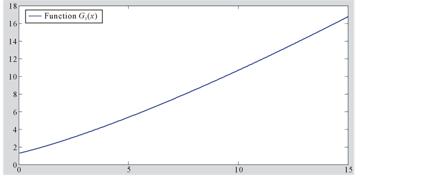
Figure 1. Graph of the function .
.
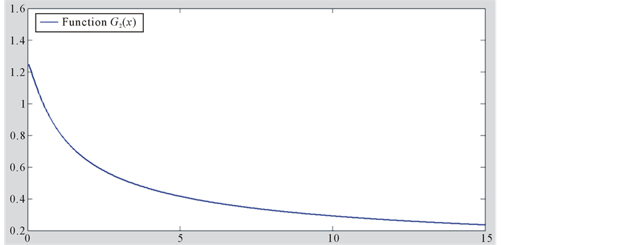
Figure 2. Graph of the function .
.
So B is the solution of the following equation:
 (2.4)
(2.4)
Lemma 2.1. The free boundary Equation (2.4) has unique positive solution B.
Proof: The Equation (2.4) is equivalent to

Denote:

The graph of
 is shown in Figure 3. We shall prove that the function
 satisfying
 ,
,
 and
and
 is decreasing and therefore the equation
 has unique solution on
 .
.
We have
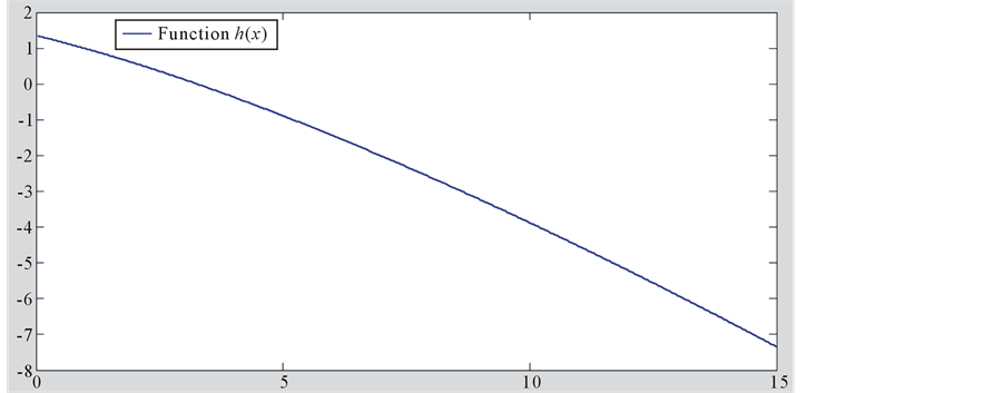
Figure 3. Graph of the function .
.

It follows that


Because

and

we obtain

We will prove that . Indeed, with the large enough x we have
 so
so

since

Consequently,
 and
and
 is decreasing so the equation
 has unique
solution on . The theorem is proved.

Theorem 2.2. Stopping time
 is the optimal stopping time for (2.1).
Proof: Let

and we will prove that

 , indeed

Now, we examine the function

Take the derivative we obtain

This follows
 .
.
Using the Dynkin’s formula to the process
 we have:
 .
.
Because B satisfying
 so the drift of Y is positive and therefore Y is super martingale and
 is martingale. By optional theorem we have:
 .
.
By
 we have
 moreover
 . So
. So .
.
We will show that B satisfy the condition: . Indeed, by general optimal stopping theory all points satisfy the form

with positive value will be in continuation area
 .
.
The optimal stopping time is the first hitting time of
 to the area:
 or
or 
Thus function G satisfy the following condition:
 .
.
We define the function:

Now, we assume , because
 is a decreasing function so
 . Then the left derivative of
 . Specially,
 with some
 . This follows
 is super martingale and
 martingale. For the stopping time
 satisfying
 we have:
 .
.
This contradicts to the existence of
 such that
 when
when

 . Finally, we achieve
 .
.
The optimal stopping time
 is the first hitting time of
 to the area
 .
.
But

 therefore
 ,
,
by this, we have finished the provement.
3. Simulation Study
To make visual for the above theory we simulate the asset price process, the posterior probability process

process
 (notice that
 is an increasing function of
 ) and the selling threshold B. Some
parameters is used in our simulating are ;
; ;
; ;
; ;
;
 and the time interval is [0, 1].
As can be seen in the figures from 4 to 8 if the price is increasing then the
 and
and
 are decreasing and conversely.
Figure 4 shows the price process has increased since the time 0.2 so the
 decreased from the respective time and it can not hit the red line denoted the threshold, therefore the optimal selling time in this case is 1.
Figure 5 simulate a price process which is fluctuated from time 0 to 0.14 and decrease dramatically at the time 0.14 so the process
 increase sharply from this and crossover the threshold, it follows that the optimal time to liquidate the asset is about 0.17. At this time the price of the asset is lower than the origin but if we hold it we will sell it at a much more loss in the future.
Another simulation is shown in Figure 6. Clearly, whenever the price process is increasing, the
 and the posterior probability process are decreasing and the liquidated time is 0.77. At this time the price is not the highest but it is significantly higher than the original value which is 1.5.
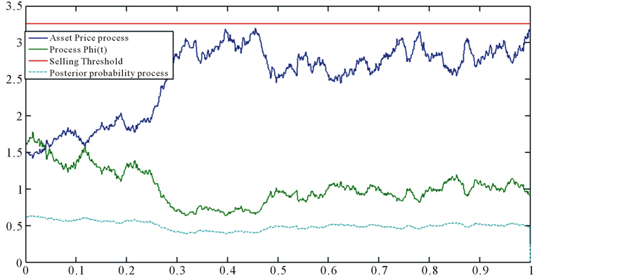
Figure 4. A simulation of asset price process, the posterior probability process, process Φ(t), the threshold probability and the optimal stopping time. In this case, the process Φ(t) always under the threshold probability so the optimal stopping time is the final time 1.
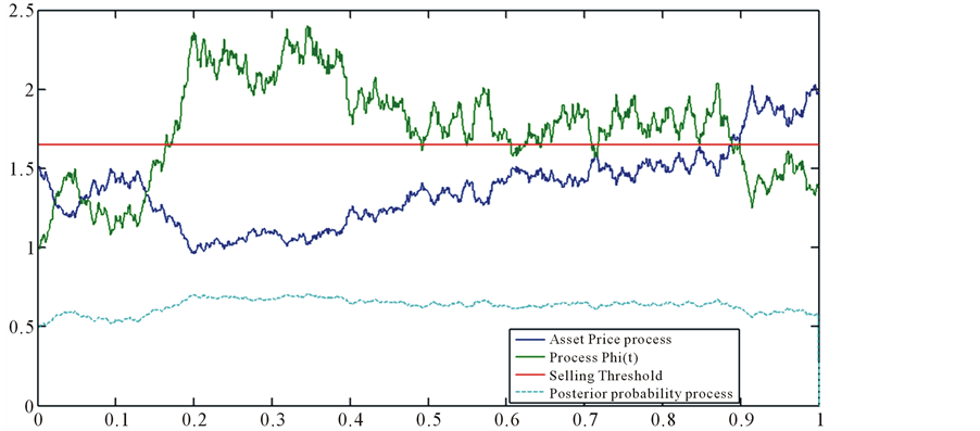
Figure 5. A simulation of asset price process, the posterior probability process, process Φ(t), the threshold probability and the optimal stopping time. In this case, the first time that the process Φ(t) over passes the threshold probability at the time 0.17 so the optimal stopping time is 0.17.
In Figure 7, we can see the same scenario with the simulation in Figure 6. The time to liquidate in this case is 0.795, the price is about 1.75 whereas the started price was 1.5. We can see
 it means that we benefit by this trade affair.
The same scenario with the simulation in Figure 1, the simulation results in Figure 8 show the price illustrates an uptrend from time 0 to the end that the process
 can not pass over the selling threshold B, consequently, the optimal time to sell in this situation is 1.
4. Conclusion
This research considers the problem of how to find the optimal time to liquidate an asset when the asset price is modeled by the geometric Brownian motion which has a change point. In particular, the drift of the process drops from a high value to a smaller one and this drift process can be modeled as two-state Markov process. The results of this research indicate that a optimal selling decision is made when the probability of downtrend surpassed some certain threshold. We also simulate the price process with a number of parameters and conduct
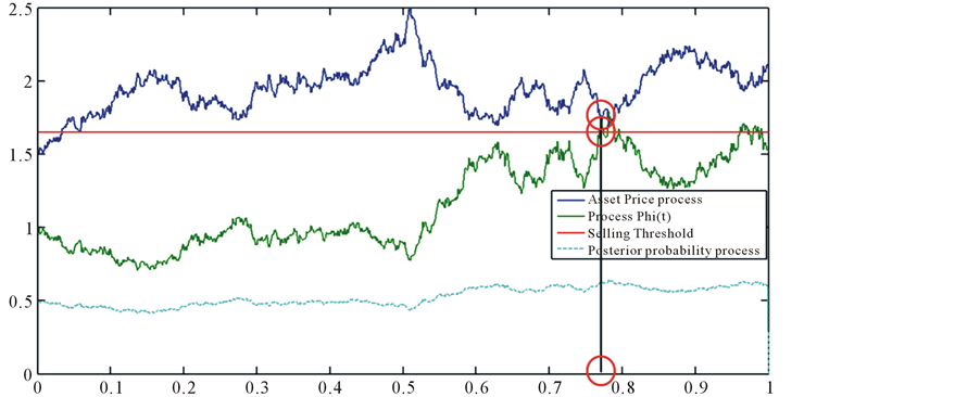
Figure 6. A simulation of asset price process, the posterior probability process, process Φ(t), the threshold probability and the optimal stopping time. In this case, the first time that the process Φ(t) over passes the threshold probability at the time 0.77 so the optimal stopping time is 0.77.
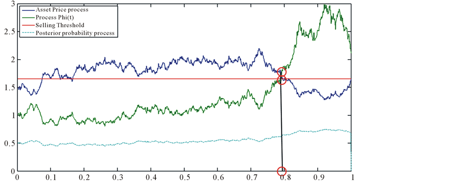
Figure 7. A simulation of asset price process, the posterior probability process, process Φ(t), the threshold probability and the optimal stopping time. In this case, the first time that the process Φ(t) over passes the threshold probability at the time 0.795 so the optimal stopping time is 0.795.
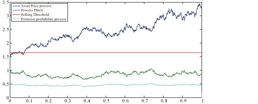
Figure 8. A simulation of asset price process, the posterior probability process, process Φ(t), the threshold probability and the optimal stopping time. In this case, the process Φ(t) always under the threshold probability so the optimal stopping time is the final time 1, the same with the case in Figure 4.
numerical solution to the experimental selling threshold. In next studies, we will consider problems in which the price growth rate is a Markov process which has more than 2 states and establish some properties as well as distribution of stopping time.
Acknowledgements
This research is funded by Vietnam National Foundation for Science and Technology Development (NAFOSTED) under grant number 10103-2012.17.
Cite this paper
PhamVan Khanh, (2015) When to Sell an Asset Where Its Drift Drops from a High Value to a Smaller One. American Journal of Operations Research,05,514-525. doi: 10.4236/ajor.2015.56040
References
- 1. Khanh, P. (2014) Optimal Stopping Time to Buy an Asset When Growth Rate Is a Two-State Markov Chain. American Journal of Operations Research, 4, 132-141.
http://dx.doi.org/10.4236/ajor.2014.43013 - 2. Khanh, P. (2012) Optimal Stopping Time for Holding an Asset. American Journal of Operations Research, 4, 527-535.
http://dx.doi.org/10.4236/ajor.2012.24062 - 3. Peskir, G. and Shiryaev, A.N. (2006) Optimal Stopping and Free-Boundary Problems (Lectures in Mathematics ETH Lectures in Mathematics. ETH Zürich (Closed)). Birkhäuser, Basel.
- 4. Shiryaev, A.N., Xu, Z. and Zhou, X.Y. (2008) Thou Shalt Buy and Hold. Quantitative Finance, 8, 765-776.
http://dx.doi.org/10.1080/14697680802563732 - 5. Guo, X. and Zhang, Q. (2005) Optimal Selling Rules in a Regime Switching Model. IEEE Transactions on Automatic Control, 9, 1450-1455.
http://dx.doi.org/10.1109/TAC.2005.854657 - 6. Lipster, R.S. and Shiryaev, A.N. (2001) Statistics of Random Process: I. General Theory. Springer-Verlag, Berlin, Heidelberg.
- 7. Shiryaev, A.N. (1978) Optimal Stopping Rules. Springer Verlag, Berlin, Heidelberg.