Abstract

This study develops the approach by Minh & Khanh [1] to the classic Barro and Sala-i-Martin method [2] , [3] named “expanded Barro regression method”, and applies this approach in analyzing the convergence of provincial per capita GDP in Vietnam over the period of 1991-2007. Different aspects of provincial convergence are considered in this paper. The estimated result on convergence from our model is compared to other models.

Keywords:Convergence, Barro Regression, Markov Model, Expanded Barro Regression

1. Introduction

Suppose that we consider as an economic variable, being a stochastic process dependent on parameter (time), (space) with considered (country) area. Observations at time (period) are known, we consider following convergent conception of economic variable

(is unlimited over time) as the convergence of function for finite value

(called “convergence state”) at sub-regions (province)

. (1)

Growth coefficient of the economic variable reveals variable rate (the variable level of a unit), variable in a unit of time at time:

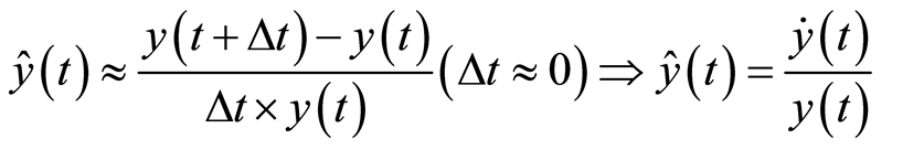. (2)

For the model (1) with assigned to income or productivity, the convergence in income and productivity is among the most-receiving attention economic issues in recent years. Many authors focused on the convergence in income, however, studying the convergence in GDP according to regions also provides many such important information.

Globally, implementing the Barro regression (see [2] -[4] ) in convergence, researches had been mentioned in many countries but only the information of the initial and final stages of the researches was analyzed. Exploiting this information at all stages was not set forth yet. In Vietnam, as the authors recognized, the implementation of classic Markov method (see [5] [6] ) in examining the convergence in income per capita and productivity growth rate hasn’t been studied yet. Therefore, this paper is designed to introduce a new method to Vietnam’s economic growth research at the region levels.

This paper develops the results of [1] and evaluates the convergence level in provinces of Vietnam (sub-regions), based on income per capita which is examined through their data on GDP, population and manpower in the period 1990-2007.

Markov method allows the researchers to monitor the movement in a distribution, and determine the invariable contribution in time at a combined level. Mixed data of the period 1990-2007 are used to calculate invariable frequency at time. This research takes a deeper consideration into whether provincial polarization in its growth leads to cluster of convergence or not. That means whether the convergence of a province group will go toward different growth rate or otherwise, a wholesale convergence will occur when all provinces move toward the same growth level. It’s necessary for a nation to analyze its convergence for the theory and policy making purpose. In the case when convergence takes shape, the policymakers will have evident to adjust the growth related variables. Additionally, the assumptions under convergence supposition can be met in a national scale because the studied units of a nation are affected by technology development, government policies, and their mobilization.

2. Theoretical Basis

2.1. Economist View of Considered Approaches

Generally, convergence results from neoclassical growth theory where for certain set of economies, their economic growth is infinitively unstable and lessening at the end, and their speed is likely to come to stationariness as production function drives downward performances by capital size. If these groups of economics have similar economic structures, they would converge at a same stable condition, narrowing the income gap. At that case, an absolute convergence occurs. However, in the case the economies have different in their structures, they witness diverse “stable conditions” and uncertain decrease in income-gap, which is called conditional convergence. This study only focuses on absolute convergence.

When analyzing a standard convergence, researchers investigate (the presence of) the convergence which presents a declining income-gap and the convergence displaying whether the poor nations witness a faster economic growth than the developed ones. It’s said that absolute convergence takes place when initial income and its later development have a negative relationship. From this theoretical economic point, the classical Barro regression models are widely implemented [2] , [3] it’s reckoned that: in the observed time, the growth pace of economic variable is defined as:

Barro Model 1  (3)

Barro Model 2    (4)

with is the initial value of economic variable; (in the Model 1) and (in the Barro Model 2) server as parameter which are estimated based on the correspondent regression equations:

(5)

(Barro Regression Equation 1)

(6)

(Barro Regression Equation 2)

with—observed error,—sub-region number (provinces, cities, localities...) survived in (nations, zones...); and is the observed value in sub-region of economic variable at the starter and in the studied time. After estimating the parameters in the above regression formula, the Neoclassical economics paradigm is employed to provide sufficient signs for variable to converge. Nevertheless, before this sign is used (when economic variable presents for income or productivity), it’s a must to check the form of Cobb-Duglass in the function for manufacturing or the concave condition of combined function for manufacture. This can’t always be achieved, especially in the Barro regression when only the information of its initial and final steps are studied. Additionally, these mentioned sufficient signs can’t help the researchers come to a certain conclusion about the inability of convergence of economic variable. Therefore, the group of authors will introduce a new method named “expanded Barro regression method” in the next 2.2-2.3 to surmount this defect. A second method: Markov method, which is usually used in published document, will be also introduced in the 2.4. This method requires the information about transitional move of the researched units included in cross-selection and temporal chain. The authors come to a conclusion that convergence takes shape if long-term forecasts for these movements go toward to 0 when forecast range increase.

In Section 3, the mentioned methods will be utilized to analyze the convergence in per capital income in Vietnam’s provinces during 1991-2007, and then to picture the typicality in the long-term tendency in the capital per income growth of Vietnam’s provinces. Section 4 for calculation outcomes show the consistence between 2 methods used in the thesis and the over-advantages of “expanded Barro regression” (compared to classic Barro regression). Section 5 for conclusion and Section 6 for acknowledgements.

2.2. Expanding Barro Regression Model

In the differential equation linguistics, to deal with problem (1), we need to build Cauchy problem responding to differential Equation (2) under form:

(7)

where is income per capita (GDP) at the beginning of research (t = 0), and represents growth rate of GDP at t. For economic thesis that economic growth rate definitely develops, where per capita growth rate negatively depends on primary income and gradually becomes lower and then convergent at stationary state at the end (if these economies have very similar structures), we consider 2 following models which is expanded from Barro models in [2] , [3] for growth rate as:

Expanding Barro 1 Model (Model 1)

(8)

Expanding Barro 2 Model (Model 2)

(9)

where A, λ > 0 are parameters.

The convergence of Model 1 was considered in [1] , in this paper we only consider the convergence of Model 2.

2.3. Expanded Regression Barro 2

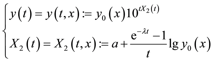
When considering Model 2, we put:

. (10)

To analyzing the Model (2) in (9), we based on (10) to get the root of (7)

. (11)

Then, it’s easy to see the form of convergence condition for the problem:

. (12)

And (11) leads to a conclusion that (12) also serves as the converging condition of problem (1). From this case and (11), we gain:

. (13)

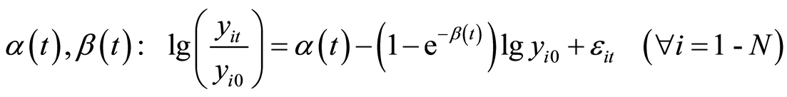
To identify the determined regression equation with parameters in the observed time, we logarit (11) and get:

(14)

by applying the next algorithm.

Algorithm 2.1. (Convergence of the Model 2)

Step 1: For each time, the researchers use (14) to set up nonlinear regression equation following parameters

. (15)

are the LS estimated of parameters the value of can be found from above regression algorithm.

Step 2: Based on (12) to test the converging condition:

a) If this algorithm isn’t true with all, problem (1) doesn’t lead to convergence, end the algorithm/process here.

b) If it’s true, for example with all value of, follow the Step 3.

Step 3: Employing (10), the estimated OLS value of the parameters can be found through:

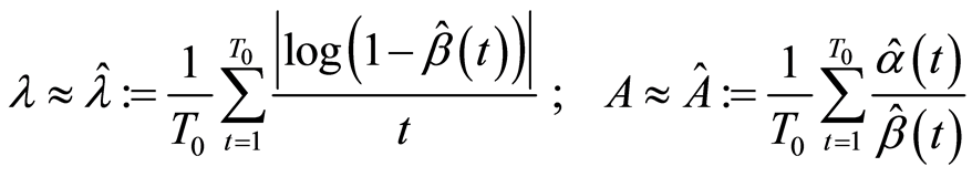(16)

is the converging speech of an economy, and (13) infers:.

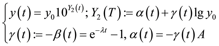
With the aim to compare the above algorithm with classic Barro Model 2 [3] , the authors initially examine this algorithm with its parameters which need to be defined in the function:

(17)

with need-to-verify variable.

When assigning the authors get of and, assigning:.

Equation (18) (Regression Barro 2) follow nonlinear and linear:

. (18)

are estimated OLS of in mentioned equations, and set:

(19)

approximate equation of (17) complying Barro 2. In order to check the errors between these 2 functions, the error of need to be checked through clause:

Lemma 2.2. If and assign

. (20)

With all we have:

. (21)

Proof. Because so we can infer the approximate value of function in (17) under

. (22)

At this value, regression Equation (18) gets close linear value (with its parameters) at:

.

For this linear regression model, the authors employ the similar methods used in (20)-(22) (replacing with). At this value (18) becomes (20) and if assign is the estimated OLS of in the above regression model, we get:.

So, from (22), we have:

. (23)

Furthermore, basing on the positive character of the matrix in (20) we get

.

Applying inequality Chebyshev:

.

We have (21). □

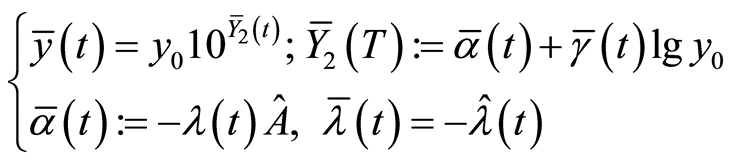
Next, we examine expanded Barro 2 with parameter, need to be defined in (11), (10) which can described as:

. (24)

With each when we put and used the rest signs of (24), we can demonstrate regression Equation (15) under linear form using parameters:

. (25)

Assigning is the estimated OLS of parameters in the above regression model (assign) and supposing that:

From this basement, we can set up simultaneous regression Equation (27)

. (26)

When we set are OLS estimated of in the above regression model we can establish approximate function of (24) following expanded Barro 2:

. (27)

Error of this approximate function can be assessed by error of function in (24), in (27), under algebraic clause:

Lemma 2.3. If the conditions of Lemma 2.2 are satisfied, with all we have:

. (28)

In the case, we can get approximate value of LS estimated in (27) by Formula (16).

Proof. It’s acknowledged that: the regression Equation (25) will be (26) with the replacement of

by, and by; the simultaneous regression Equation (26) coincide with (27). Therefore, when reiterating the demonstrations of Lemma 2.2 (with the replacement of by), we get the result of the observing lemma. In this situation, Formula (28) has its form as (29). □

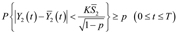
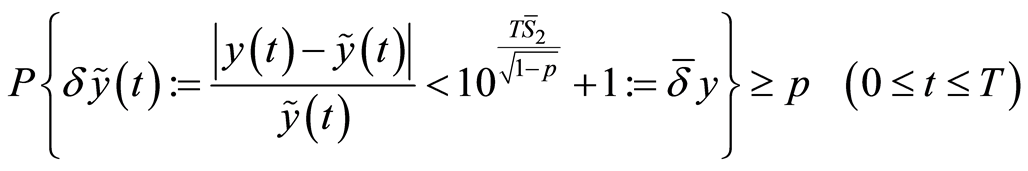
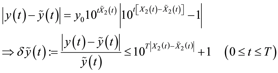
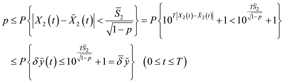
Finally, in order to the higher accuracy of the expanded Barro 2 (compared to coefficient classic one), we provide the same outcome to Theorem 2.4.

Theorem 2.4. If and, we can evaluate relative error of approximate function (19) (based on classic Barro) and (17) (under expanded Barro 2) from following algorithm:

(29)

(30)

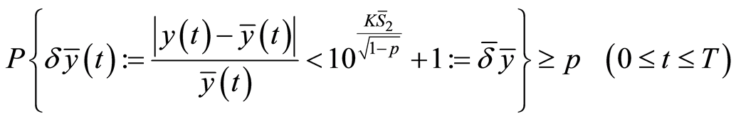
with. In addition, if, and reliable p; the higher value of relative error between it in classic Barro 2 and in expanded Barro 2 is defined as:

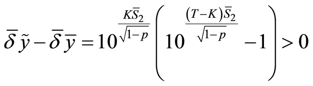(31)

with

Proof. From (17) and (19), we find out:

.

And then, (21) we infer:

.

At this point, (29) is proved. In a similar method, (24) and (27) lead to:

.

From this result and (65), we have:

so we get (30).

Finally, because... of in (29), we can easily find out: from expression in (29) from expression (in (29)) and (in (30)) we have (31).

Noticing that terms in above expression are introduced to defined the applying range of the (31)’s result. When doing algebraics, we need to choose (in possible condition) in order to allow approximate function (in (17)) to converge under probability of function (in (24)). □

2.4. Markov Chain Models

The method of Markov chain using in convergence problem was presented in [1] , we do not present this content again.

3. Experimental Estimating Results

Barro 1 Model:

Set independent variables are growing logarithm of per capita income in the province at late, and dependent ones represent income per capita at early stages. After removing inappropriate variables, final estimation for the period of 1990-2007 is as:

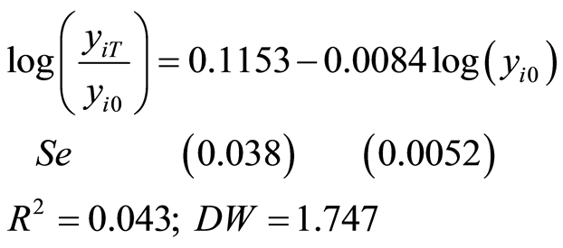
Estimated results shows that negative coefficient β have no 10% lower significance level 11%. We also split into small periods to estimate above equation but no ones see coefficient β statistically better than that of the whole period 1990-2007.

Barro 2 Model:

Apply empirical equations drawn from neoclassical theory to Vietnam with the whole researching period of 1990-2007, estimating models will be classified via following intervals: model (2a) for 1990-1996, model (2b) over the time of 1997-2001, from 2002 to 2007 is represented by model (2c), and the last and model (2d) estimates total sample period. We used mixed data for estimation.

Estimate method using panel data but we are just saying in case of fixed effects (stochastic effects) should not fear the wrong when we added from the fixed effect on it.

Table 1 displays estimating results for above 4 models.

We all know that growth rate of some economy depends negatively on its primary income and goes down for decreasing disparity between its steady—state returns and net income as in researching process, this suggests that results in convergence. See results from Table 1, just two periods of 1990-1996 and 2002-2007 are convergent with annual speed of 0.010966 and 0.001536 respectively.

Expanding Barro 1 Model:

From above theoretical models and per capita income data of 59 provinces over Vietnam, we used analysis of regression to analyze the convergence of economic variable provincial per capita GDP. For each period (year), we build 17 regression equations by virtue of cross data:

.

For these equations, we obtains the set of estimated values for parameters as follow

and value

.

Average earnings at convergent state is.

We can use following model to forecast average income in coming years:

.

We obtain forecasted results as in Table2

Here, we denote is estimator for.

Expanding Barro 2 Model:

For the expanding Barro 2 Model, we consider following 17 regression equations as well:

.

These equations result in the estimator set of parameters as in Table3

Estimators for and as:

.

Estimator for average income at convergent state is:

.

We also use following equation to forecast per capita income in the future:

.

We obtain estimation results as in Table4

Table 5 shows average standard deviation values of and responding to the two regression equations.

Convergence has been obtained in need of respective 600 and 500 years for these responding Barro Models since 1990.

Markov Chain Model:

Experimental results of per capita income convergence problems by Markov chains method has been presented in [6] . Here we will compare the results obtained to the problem of per capita income convergence in the model of Barro regression, Barro extended regression model and Markov chain model.

4. Comparison between Models

Attaching the same data set N = 59, T = 17 of Vietnam’s provinces within 1991-2997, we found that the results calculated under the Algorithm 2.1 in [1] and Algorithm 2.1 in this paper share the general point with Markov chain algorithm in the fact that the results indicate the common characteristic, the convergence of the Model 2.

However, if using classic Barro models for the same data set, we have not yet found common characteristics mentioned above. This is also explained by Theorem 2.3 in [1] and Theorem 2.4 in this paper related to the lack of accuracy in classic Barro models compared to corresponding extended models.

5. Conclusions

This research has used different methods to study the income convergence of Vietnam’s provinces in 1990-2007. Results from extended Barro model are consistent with the results under approaching method based on Markov chains and it has been proved that the error from extended models is smaller than that from classic Barro models.

With current situation and no change in policy and regime, according to Model 1, Vietnam’s income per capita is about 80,000 USD/year; this is an impressive figure and also the expectations of every citizen in Vietnam.

Estimation result from Markov chain model indicates convergence signs in distribution. The reason might be obstacles in regime which slow down technology transition process leading to limited mobility. Moreover, the lack of necessary infrastructure and unfair distribution causes technology diffusion to slow down. The speed of this process may vary among provinces.

Acknowledgements

This research is funded by Vietnam National Foundation for Science and Technology Development (NAFOSTED) under grant number II 2.2-2012-18.

References

- Minh, N. and Khanh, P. (2013) Forecasting the Convergence State of per Capital Income in Vietnam. American Journal of Operations Research, 3, 487-496. http://dx.doi.org/10.4236/ajor.2013.36047
- Barro, R.J. and Sala-i-Martin, X. (1991) Convergence across States and Regions. Brookings Papers on Economic Activity, 1, 107-158. http://dx.doi.org/10.2307/2534639
- Barro, R.J. and Sala-i-Martin, X. (1995) Economic Growth. McGraw-Hill, New York.
- Sala-i-Martin, X. (1996) The Classical Approach to Convergence Analysis. The Economic Journal, 106, 1019-1036. http://dx.doi.org/10.2307/2235375
- Quah, D.T. (1993) Empirical Cross-Section Dynamics in Economic Growth. European Economic Review, 37, 426-434. http://dx.doi.org/10.1016/0014-2921(93)90031-5
- Bernard, A.B. and Jones, C.I. (1996) Comparing Apples to Oranges: Productivity Convergence and Measurement across Industries and Countries. American Economic Review, 86, 1216-1238.